
Fig. 1
Fig. 2
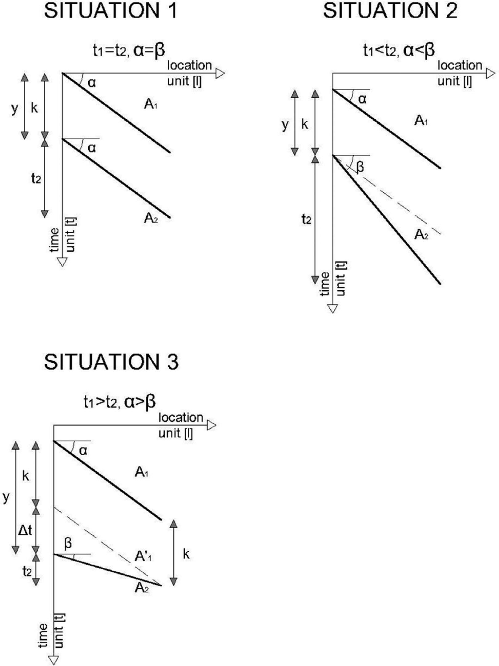
Fig. 3
Fig. 4
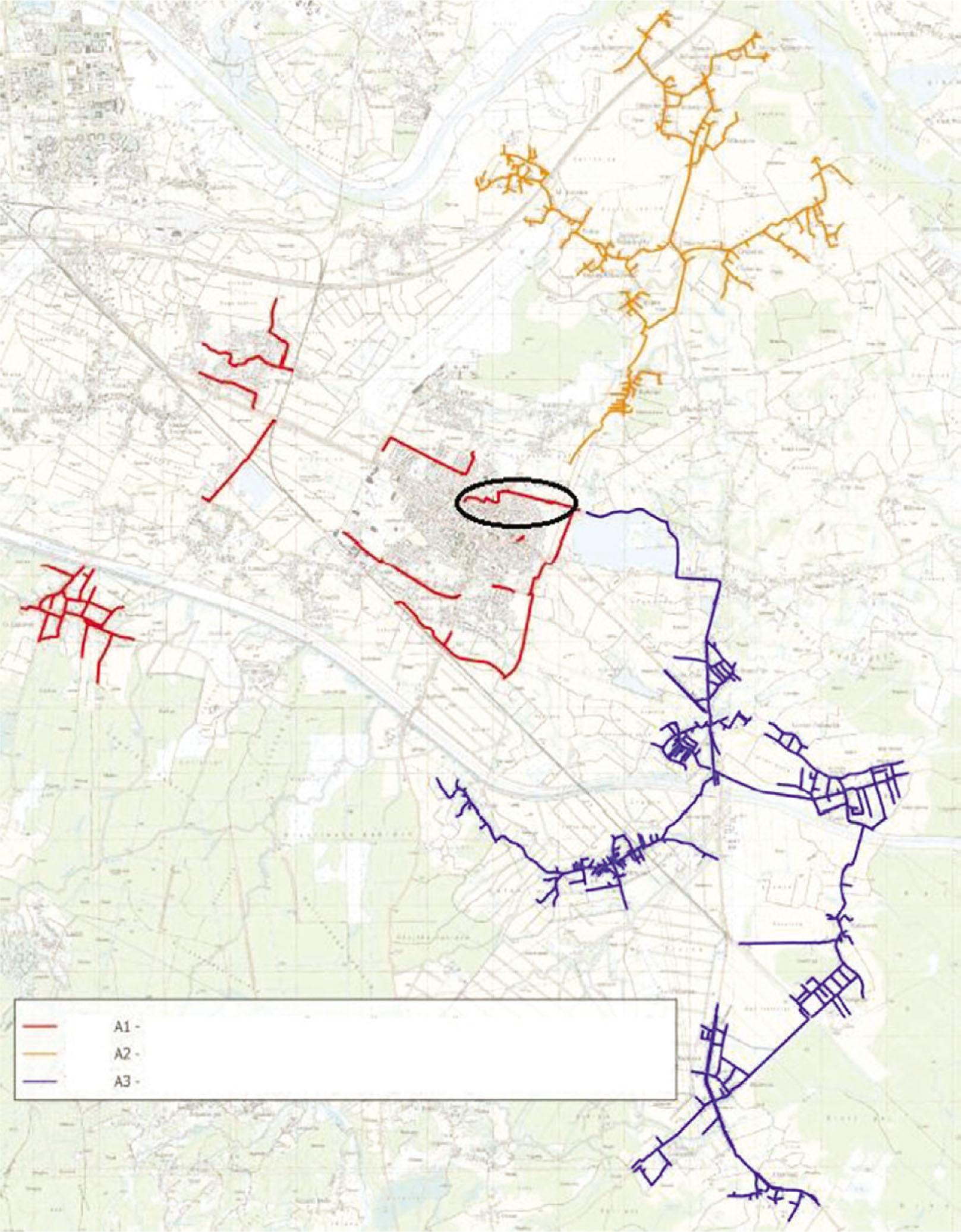
Fig. 5
Leading activities and their related variables of another pipeline project from the same sewer system
| Leading activities | ΔQ | Up | Δl | α, β (tan−1) | ta (days) | Task link | k | y | |
|---|---|---|---|---|---|---|---|---|---|
| 1 | Pulverizing and grinding of existing roadway asphalt or concrete curtain | 4500 | 292.08 | 2113 | 0.0073 | 16 | F-F | 1 | 8 |
| 2 | Mechanical excavation | 5653.52 | 669.76 | 2113 | 0.0040 | 9 | F-F | 1 | 7 |
| 3 | Manual excavation | 1413.38 | 669.76 | 2113 | 0.0010 | 3 | F-F | 0 | 2 |
| 4 | Replacement of low foundation material | 559.98 | 878.40 | 2113 | 0.0003 | 1 | S-S | 1 | 1 |
| 5 | Trimming, leveling, and grading the landfill base | 1610 | 2927.9 | 2113 | 0.0003 | 1 | S-S | 1 | 1 |
| 6 | Spreading filter pedestrian finishing base | 209 | 878.40 | 2113 | 0.0001 | 1 | S-S | 1 | 1 |
| 7 | Installation of manholes | 133 | 2.00 | 2113 | 0.0197 | 42 | S-S | 0 | 0 |
| 8 | Lowering pipe into trench | 2113.6 | 36.40 | 2113 | 0.0275 | 59 | F-F | 1 | 58 |
| 9 | Spreading rounded gravel above the pipes | 1071.1296 | 878.40 | 2113 | 0.0006 | 2 | S-S | 1 | 1 |
| 10 | Backfill | 2480 | 1152.9 | 2113 | 0.0010 | 3 | F-F | 1 | 2 |
| 11 | Embankment-road compacting | 2080 | 1112.6 | 2113 | 0.0009 | 2 | S-S | 1 | 1 |
| 12 | Base pavement-base course layer | 5195 | 1145.4 | 2113 | 0.0021 | 5 | S-S | 1 | 1 |
| 13 | Surface pavement-binder and wearing course | 5195 | 1145.4 | 2113 | 0.0021 | 5 | |||
| Total time: 88 days | |||||||||
Linear continuous activities of the analyzed pipeline project and their related variables
| Leading activities | First three variables determined from technical documentation | ||||||||
|---|---|---|---|---|---|---|---|---|---|
| ΔQ | Up | Δl | α, β (tan−1) | tn (days) | Task link | k | y | ||
| 1 | Pulverizing and grinding of existing roadway asphalt or concrete curtain | 2662.807 | 292.08 | 920 | 0.009909 | 10 | F-F | 1 | 6 |
| 2 | Mechanical excavation | 2949.962 | 669.76 | 920 | 0.004787 | 5 | F-F | 1 | 4 |
| 3 | Manual excavation | 737.49 | 669.76 | 920 | 0.001199 | 2 | F-F | 0 | 1 |
| 4 | Replacement of low foundation material | 474.896 | 878.40 | 920 | 0.000588 | 1 | S-S | 1 | 1 |
| 5 | Trimming, leveling, and grading of the landfill base | 1637.047 | 2927.9 | 920 | 0.000608 | 1 | F-F | 1 | 1 |
| 6 | Spreading filter pedestrian finishing base | 248.39 | 878.40 | 920 | 0.00030 | 1 | S-S | 1 | 1 |
| 7 | Installation of manholes | 47 | 2.00 | 920 | 0.012771 | 24 | S-S | 0 | 0 |
| 8 | Lowering of pipe into trench | 849.38 | 36.40 | 920 | 0.025358 | 24 | F-F | 1 | 23 |
| 9 | Spreading rounded gravel above the pipes | 1273.79 | 878.40 | 920 | 0.001576 | 2 | S-S | 1 | 1 |
| 10 | Backfill | 2815.45 | 1152.9 | 920 | 0.002654 | 3 | F-F | 1 | 3 |
| 11 | Embankment-road compacting | 941.31 | 1112.6 | 920 | 0.000920 | 1 | S-S | 1 | 1 |
| 12 | Base pavement-base course layer | 2344.797 | 1145.4 | 920 | 0.002225 | 3 | S-S | 1 | 1 |
| 13 | Surface pavement-binder and wearing course | 2344.797 | 1145.4 | 920 | 0.002225 | 3 | |||
| Total time | 46d | ||||||||
The equations for calculation of time buffer and duration of two adjacent activities
| Situation 1. α = β | Situation 2. α < β |
| Situation 3. α > β | |
Comparison of the new LSM-based method for time estimation with the two existing methods
| Integrated CPM–LOB model (Ammar, 2013) | PSM (Lucko, 2007, 2008) | LSM-based method for early time estimation |
|---|---|---|
| 1) LOB calculations | 1) Initial equations | 1) Activity list |
| 2) Calculating activity duration | 2) Buffer equations | 2) Calculating activity durations and slopes |
| 3) Specifying logical relationships using overlapping activities (buffer time) | 3) Initial stacking | 3) Using the newly developed algorithm for determination of buffers between activities |
| 4) Time scheduling | 4) Minimum differences | 4) Using the newly developed algorithm for calculation of project duration |
| 5) Criticality analysis | 5) Differentiation | |
| 6) Final consolidation | ||
| 7) Criticality analysis |
Time–cost performance for civil engineering projects in the expanded Hong Kong sample
| Project type | K | B | R | Total projects |
|---|---|---|---|---|
| Total civil works | 250.5 | 0.206 | 0.79 | 148 |
| Roadworks | 251.2 | 0.225 | 0.87 | 57 |
| Other civil works | 262.5 | 0.185 | 0.69 | 91 |