
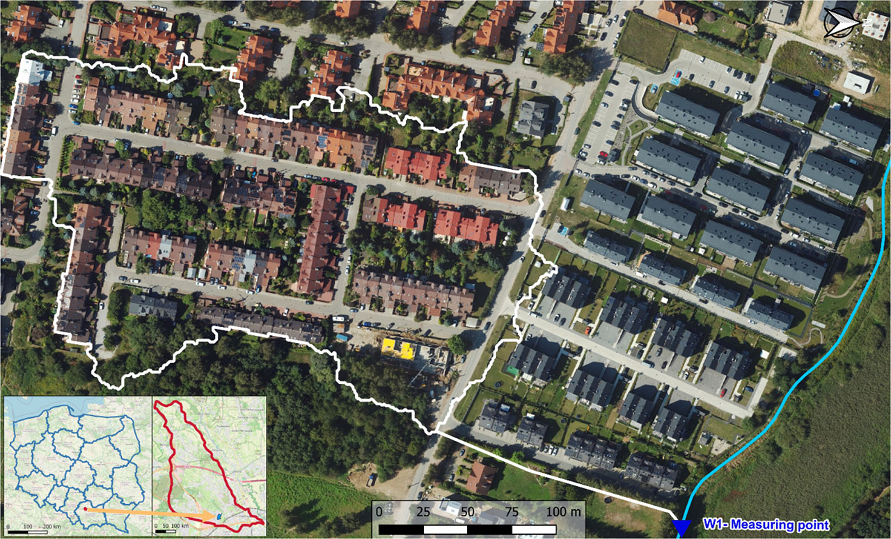
Figure 1.
Location of the measuring point in the study area with catchment for the existing outfall W1
Table 1.
Analyzed scenarios
| Scenario S0 | Scenario S1 | Scenario S2 | Scenario S3 | Scenario S4 | Scenario S5 | Scenario S6 | Scenario S7 | |
|---|---|---|---|---|---|---|---|---|
| Precipitation duration | 90 min (4.2 mm) | 15 min | 30 min | 45 min | 60 min | 90 min | 120 min | 180 min |
| Average rainfall intensity [LPS/ha]* | 7.8 | 273.32 | 175.33 | 134.52 | 105.37 | 74.81 | 59.55 | 42.46 |
| Total precipitation p = 10% [mm] | 4.2 | 24.60 | 31.56 | 36.32 | 37.93 | 40.40 | 42.88 | 45.86 |
| Precipitation intensity p = 10% [mm/hr] | 2.80 | 98.40 | 63.12 | 48.43 | 37.93 | 26.93 | 21.44 | 15.29 |
Table 2.
Spatial analyses based on the Database of Topographical Objects of the study area
| Land use | Area | |
|---|---|---|
| ha | % | |
| Roofs | 1.12 | 26.9 |
| Roadways, pavement, alleys | 0.40 | 9.6 |
| Single- and multi-family residential land | 2.17 | 52.0 |
| Biologically active areas | 0.48 | 11.5 |
| TOTAL | 4.17 | 100.0 |
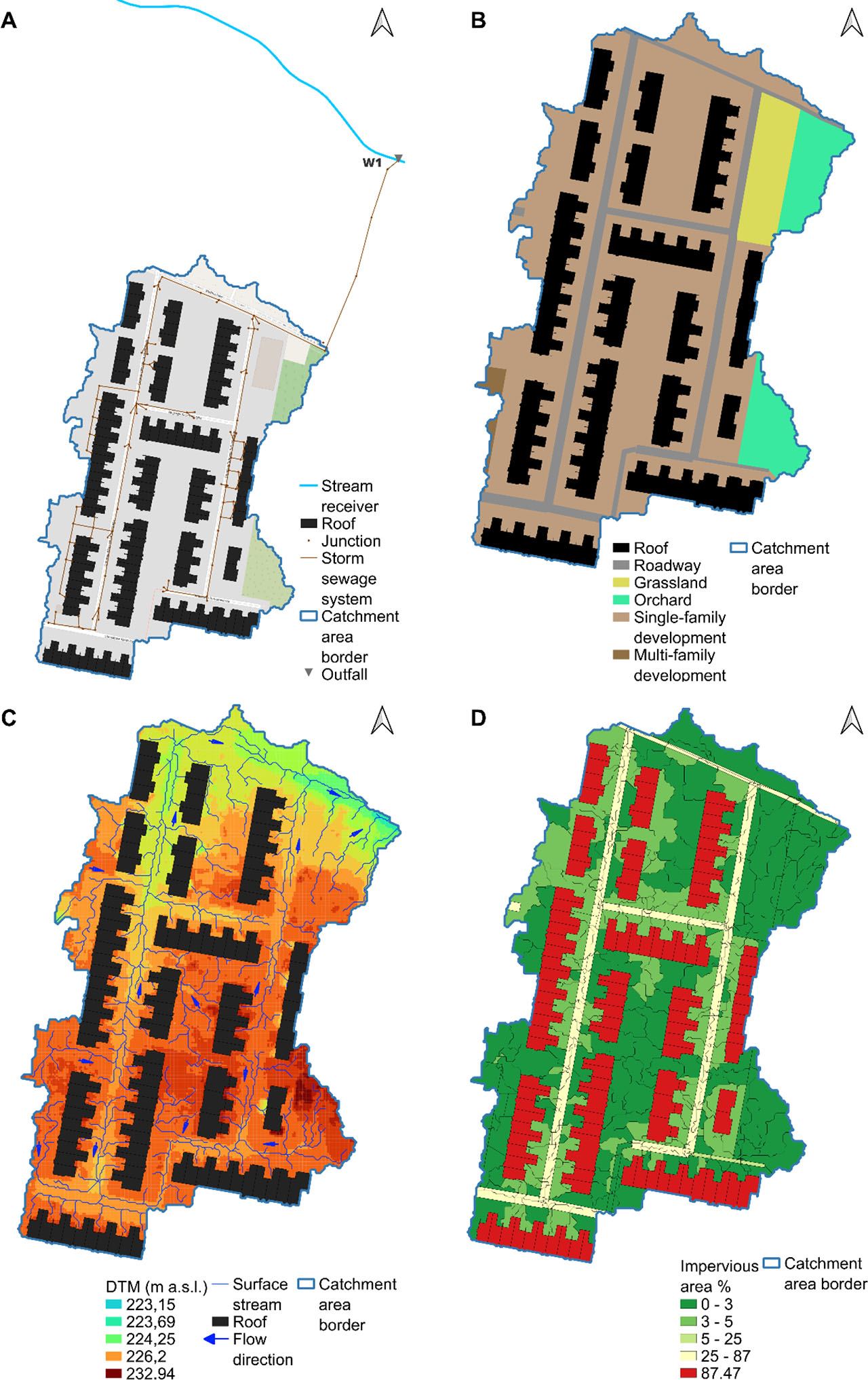
Figure 2.
Results of detailed analyses of the study area using available databases: A — route of the drainage system; B — land use; C — elevation and directions of surface water runoff; D — subcatchment imperviousness
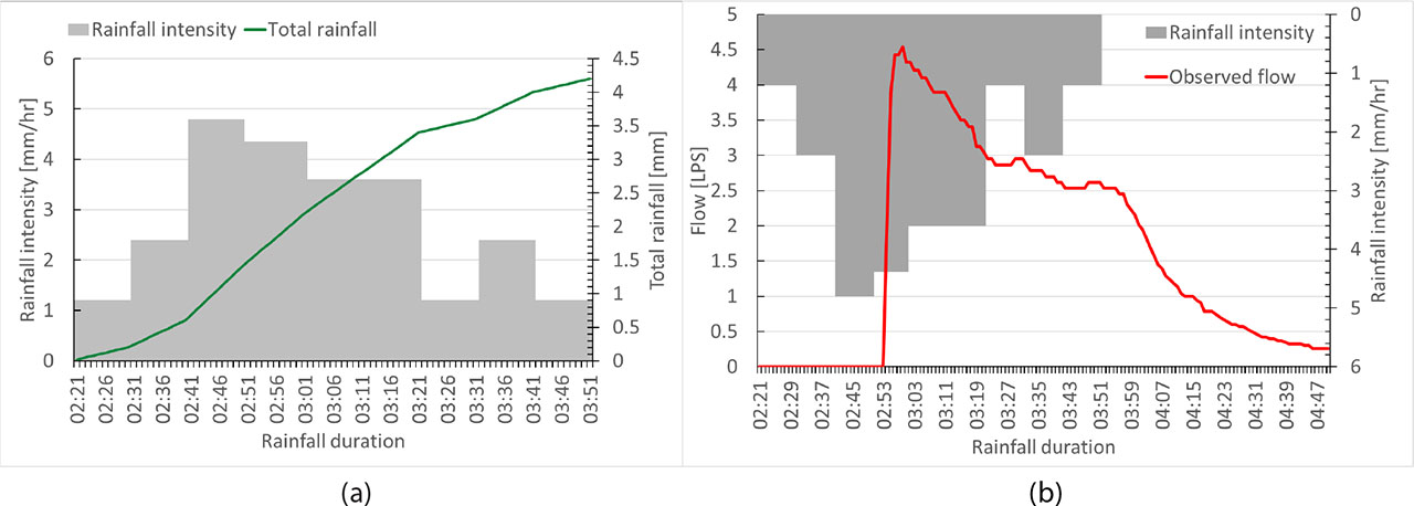
Figure 3.
Rainfall mass curve and hyetograph of 4.2 mm precipitation (a) and flow observed at outfall W1 (b) used for the calibration process
Table 3.
Values of the basic parameters for the land use groups in the study area obtained during the SWMM calibration process
| Description | Imperv [%] | N Imperv | N Perv | Dstore Imperv [mm] | Dstore Perv | Zero Imperv [%] | Width | |
|---|---|---|---|---|---|---|---|---|
| min | max | [mm] | A [m] | |||||
| Building roofs-BUBD | 87.47 | 0.010 | 0.045 | 3.69 | 3.69 | 36.00 | 0.7 | |
| Other roadway-SKJZ08 | 13.1 | 36.0 | 0.015 | 0.300 | 1.20 | 5.08 | 40.00 | 0.3 |
| Local roadway-SKJZ06 | 34.6 | 49.5 | 0.010 | 0.300 | 1.20 | 5.08 | 40.00 | |
| Alley-SKRP01 | 2.0 | 3.2 | 0.011 | 0.280 | 1.20 | 5.08 | 40.00 | |
| Grass vegetation-PTTR01 | 1.0 | 2.5 | 0.140 | 0.280 | 5.08 | 7.62 | 20.00 | 0.3 |
| Orchard-PTUT03 | 1.1 | 2.88 | 0.210 | 0.280 | 5.08 | 7.62 | 20.00 | |
| Single-family dwelling-PTZB02 | 2.0 | 4.02 | 0.105 | 0.280 | 5.08 | 7.62 | 20.00 | |
Table 4.
The basic measures of fitness coefficients for built SWMM model
| Indicator | Description | Formula | Obtained value | Assessment | Literature | |
|---|---|---|---|---|---|---|
| NSEC | Nash-Sutcliffe Efficiency Coefficient | Compare the results of model’s response and measurement data | 0.885 | -∞ - 1; very good | [Titterington et al. 2017], [Moriasi et al. 2007], [Lin et al. 2017] | |
| ISE | Integral Square Error | The accuracy of the matching between simulated and observed data | 0.02 | 0 – 3; excellent | [Shamsi et al. 2017] | |
| RMSE | Root Mean Square Error | Differences between observed and simulated values | 0.442; < 0.5*1.307 | less than half of the standard deviation; good | [Singh et al. 2004], [Moriasi et al. 2007] | |
Table 5.
Summary of the LID parameters used in the calibrated SWMM model according to [Bond et al. 2021]
| Layer | Parameter | Unit | Bio-retention cells (BC) |
|---|---|---|---|
| Surface layer | Berm height | mm | 250 |
| Vegetation volume | share | 0.1 | |
| Surface roughness | – | 0.3 | |
| Surface slope | % | 1 | |
| Swale Side Slope | run/rise | – | |
| Soil layer | Thickness | mm | 600 |
| Porosity | share vol. | 0.45 | |
| Field capacity | share vol. | 0.121 | |
| Wilting point | share vol. | 0.057 | |
| Conductivity | mm/hr | 91 | |
| Conductivity slope | – | 44 | |
| Suction head | mm | 50 | |
| Storage layer | Thickness | mm | 400 |
| Void ratio | voids/solids | 0.54 | |
| Seepage rate | mm/hr | 2.6 | |
| Clogging factor | – | 0 | |
| Drain | Flow coefficient | mm/hr | 5.4* |
| Drain exponent | – | 0.5 | |
| Offset height | mm | 200 |
* The parameter was calculated using formula (3)
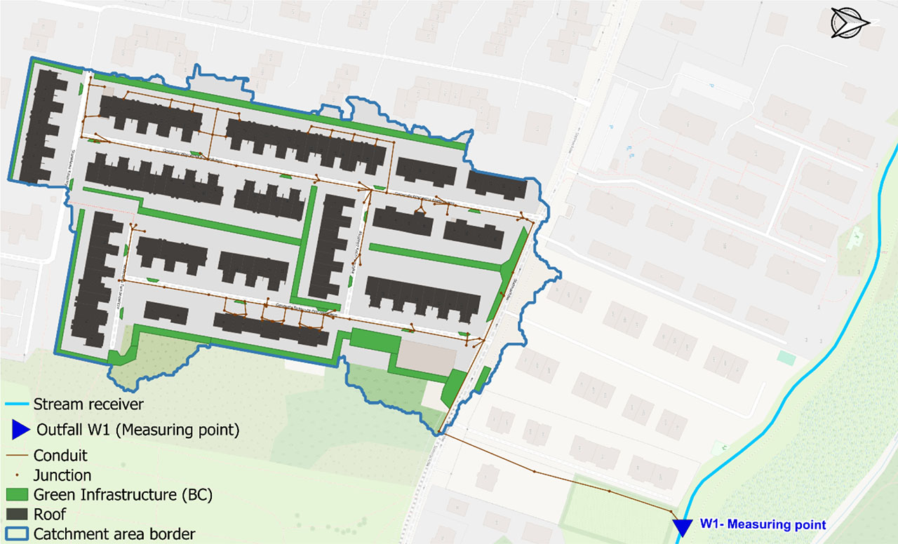
Figure 4.
Illustration of the implementation of green infrastructure (BC) in the study area of an existing housing estate.
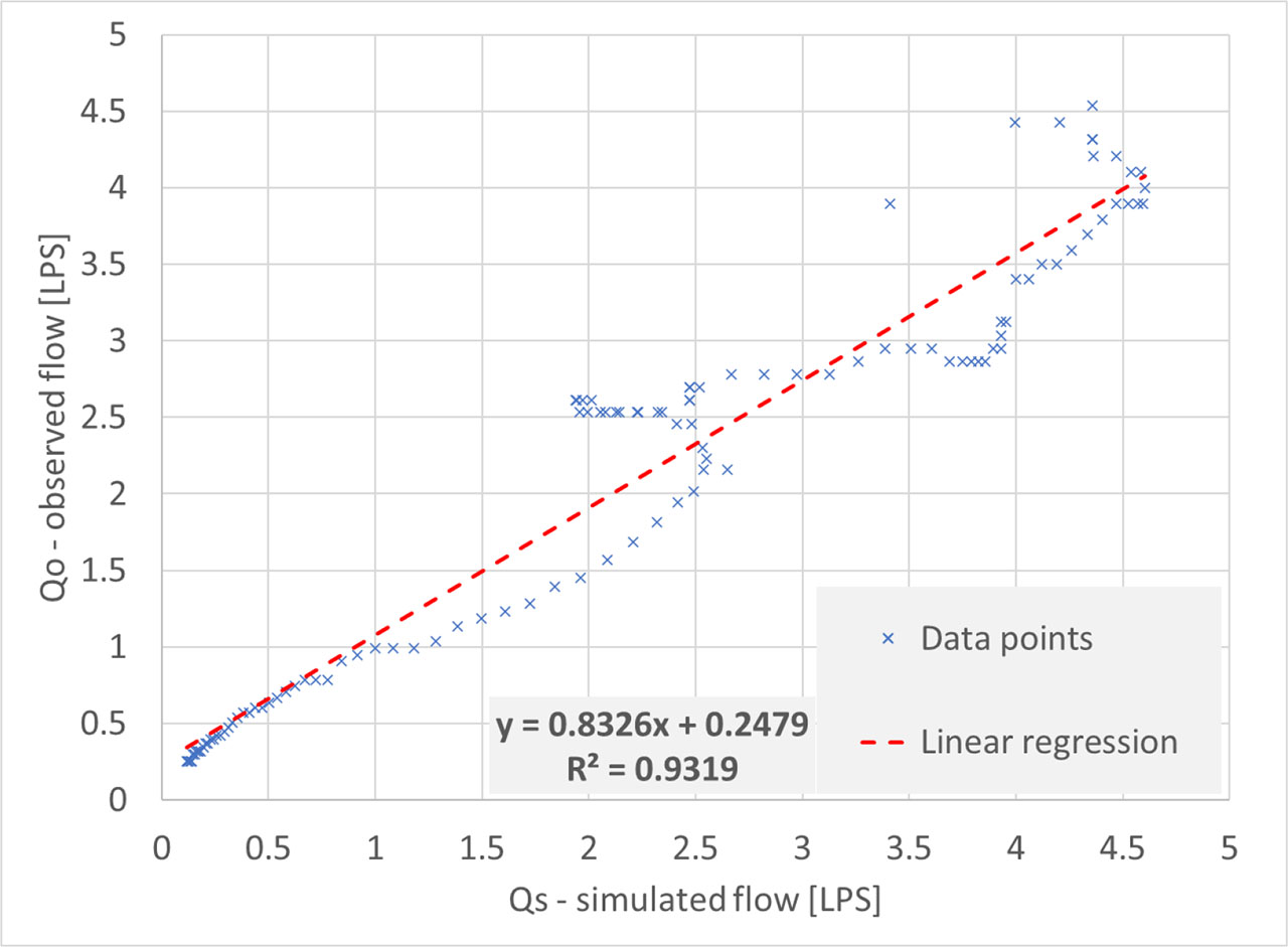
Figure 5.
Linear regression plot of R2 for a dataset of the measured rainwater flow (Qo) at outfall W1 and the simulated value (Qs) based on the SWMM
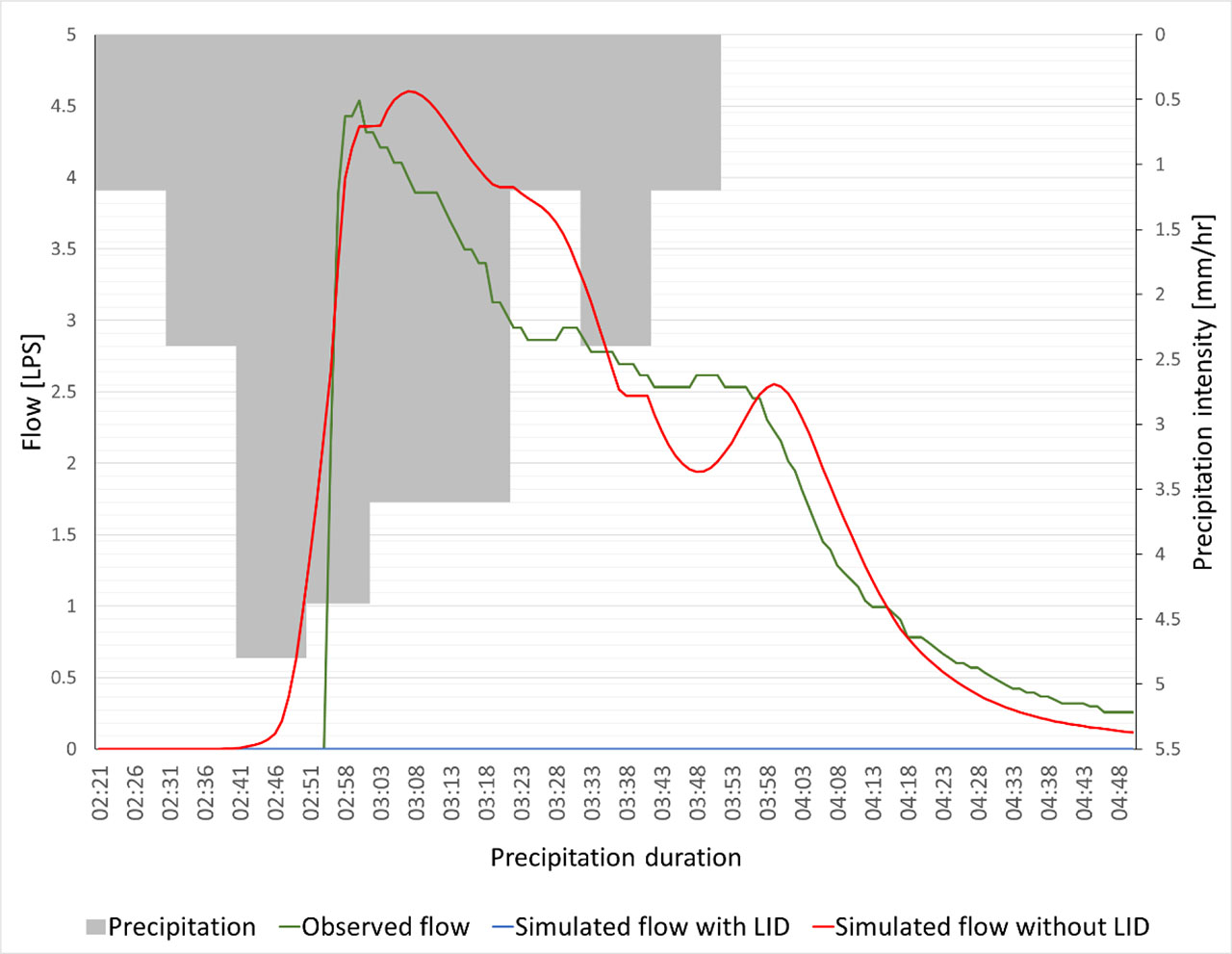
Figure 6.
Flow observed at outfall W1 on August 26, 2023, along with the modelling results for the existing conditions, and for the scenario with the selected LID equipment implemented
Table 6.
The simulation results of the calibrated model for the entire study area at the sewer outfall for scenarios S0–S7
| Scenario S0 | Scenario S1 | Scenario S2 | Scenario S3 | Scenario S4 | Scenario S5 | Scenario S6 | Scenario S7 | |
|---|---|---|---|---|---|---|---|---|
| no LID | ||||||||
| Max flow [LPS] | 4.6 | 449.2 | 464.0 | 454.8 | 393.1 | 359.3 | 349.9 | 266.2 |
| Total volume [m3] | 17 | 539 | 752 | 916 | 953 | 1008 | 1072 | 1139 |
| with LID | ||||||||
| Max flow [LPS] | 0.0 | 17.5 | 31.6 | 31.7 | 25.2 | 22.6 | 22.1 | 17.6 |
| Total volume [m3] | 0 | 29 | 56 | 111 | 134 | 167 | 204 | 246 |
| reduction | ||||||||
| Max flow [LPS] | 100% | 96% | 93% | 93% | 94% | 94% | 94% | 93% |
| Total volume [m3] | 100% | 95% | 93% | 88% | 86% | 83% | 81% | 78% |
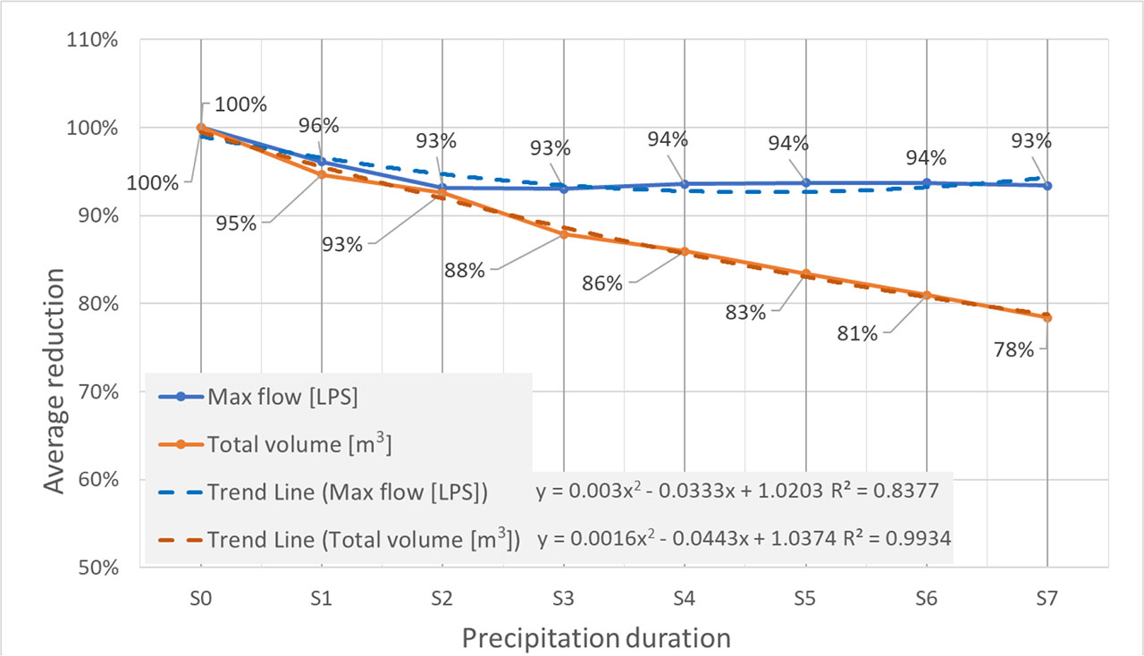
Figure 7.
Average reductions in the total volume and peak flow for scenarios S0–S7
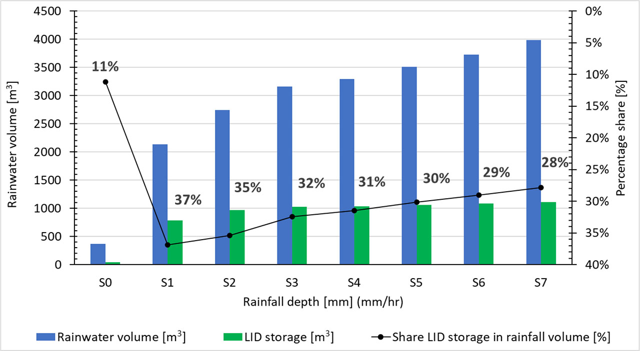
Figure 8.
Percentage distribution of the rainwater volume and storage volume of LID facility as a function of rainfall depth
Table 7.
Summary of the simulation results of the calibrated SWMM for individual LID facilities implemented in the study area for scenarios S0–S7
| Scenario | S0 | S1 | S2 | S3 | S4 | S5 | S6 | S7 |
|---|---|---|---|---|---|---|---|---|
| Total Inflow (m3) | 37.9 | 658.2 | 987.1 | 1234.8 | 1304.7 | 1404.0 | 1512.8 | 1629.2 |
| Surface and Drain Outflow (m3) | 0.0 | 32.7 | 133.6 | 273.6 | 318.7 | 385.4 | 458.9 | 538.8 |
| Average inflow (L/m2) | 0.008 | 0.139 | 0.208 | 0.260 | 0.275 | 0.296 | 0.319 | 0.344 |
| Average outflow (L/m2) | 0.000 | 0.007 | 0.028 | 0.058 | 0.067 | 0.081 | 0.097 | 0.114 |
| Average reduction (%) | 100 | 95 | 86 | 78 | 76 | 73 | 70 | 67 |
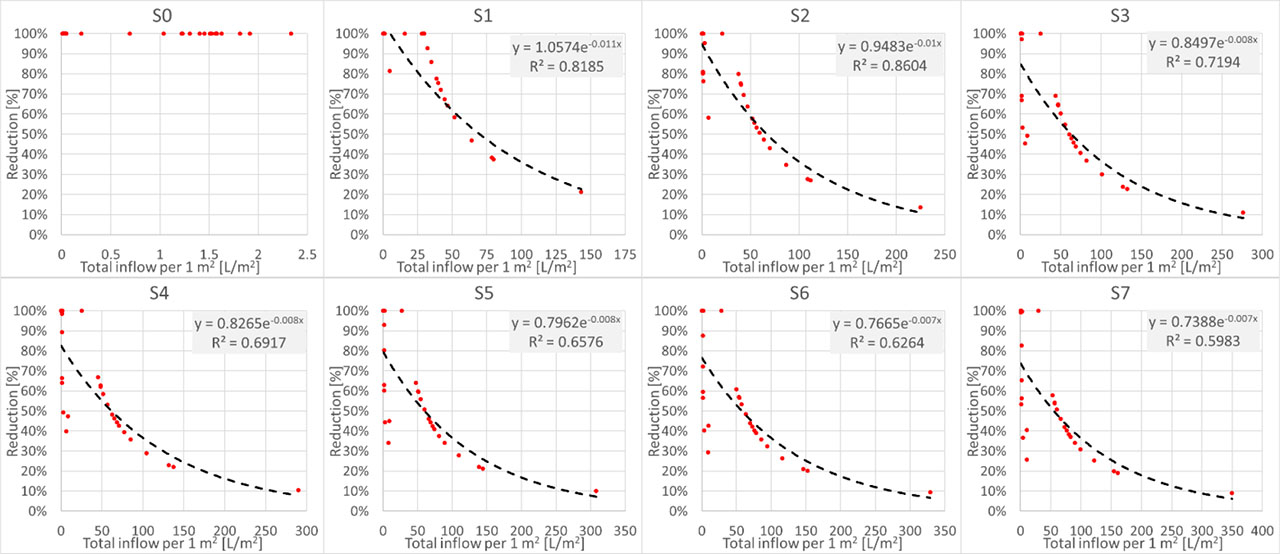
Figure 9.
Dependence of the total inflow per 1 m2 and reduction in rainwater for BC cells in the residential area under study for scenarios S0–S7
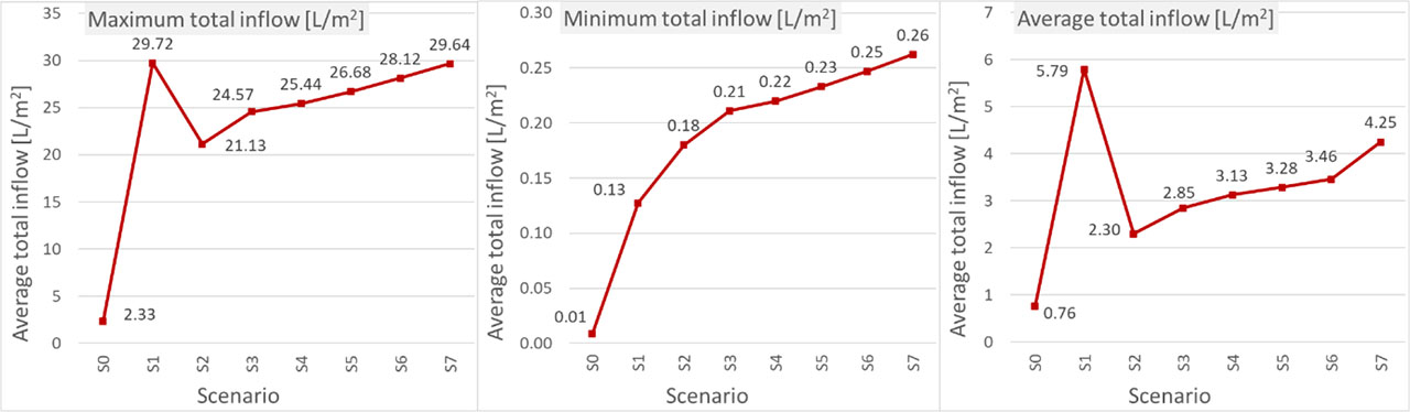
Figure 10.
Maximum, minimum and average values of the rainwater inflow limit [L/m2] per 1 m2 of surface area of LID facilities for scenarios S0–S7 for which there was a 100% quantitative reduction of inflow
Table 8.
Summary of the results obtained for the considered precipitation scenarios S0–S7
| No. | Scenario | S0 | S1 | S2 | S3 | S4 | S5 | S6 | S7 |
|---|---|---|---|---|---|---|---|---|---|
| share LID storage in rainfall volume | |||||||||
| 1A | Rainwater volume [m3] | 365 | 2137 | 2742 | 3156 | 3296 | 3510 | 3725 | 3984 |
| 1B | Final LID storage [m3] | 41 | 788 | 970 | 1024 | 1036 | 1057 | 1081 | 1108 |
| 1 | Average share [%] | 11% | 37% | 35% | 32% | 31% | 30% | 29% | 28% |
| LID hydrological performance | |||||||||
| 2A | Average inflow [L/m2] | 0.008 | 0.139 | 0.208 | 0.260 | 0.275 | 0.296 | 0.319 | 0.344 |
| 2B | Average outflow [L/m2] | 0.000 | 0.007 | 0.028 | 0.058 | 0.067 | 0.081 | 0.097 | 0.114 |
| 2 | Average reduction [%] | 100% | 95% | 86% | 78% | 76% | 73% | 70% | 67% |
| average total inflow to LID with full reduction | |||||||||
| 3 | Fully reduced inflow [L/m2] | 0.76 | 5.79 | 2.30 | 2.85 | 3.13 | 3.28 | 3.46 | 4.25 |
| total outfall volume reduction | |||||||||
| 4A | Total volume [m3] | 17 | 539 | 752 | 916 | 953 | 1,008 | 1,072 | 1139 |
| 4B | Reduced volume [m3] | 0 | 29 | 56 | 111 | 134 | 167 | 204 | 246 |
| 4 | Average reduction [%] | 100% | 95% | 93% | 88% | 86% | 83% | 81% | 78% |
| outfall peak flow reduction | |||||||||
| 5A | Peak flow [LPS] | 4.60 | 449.16 | 464.03 | 454.78 | 393.10 | 359.34 | 349.85 | 266.20 |
| 5B | Reduced peak flow [LPS] | 0.00 | 17.51 | 31.63 | 31.66 | 25.19 | 22.57 | 22.05 | 17.58 |
| 5 | Average reduction [%] | 100% | 96% | 93% | 93% | 94% | 94% | 94% | 93% |