
Table 1
Analysis of covariance (separate slopes model) of log10 SST and log ejaculate investment in the male age tactic with the covariate log soma mass and after the removal of the interaction term (reduced model)
| Source | df | Mean square | F | Beta (tactic x soma) | SE Beta | p |
|---|---|---|---|---|---|---|
| Model SST | 3 | 0.071 | 109.75 | 6.485 | 0.848 | 0.000 |
| Model EI | 3 | 5.844 | 3.759 | −2.428 | 2.756 | 0.026 |
| Age x soma | 4 | 0.999 | 17.62 | (0.133; 0.318) | 1.061; 3.448) | 0.000 |
| Error SST | 22 | 0.0001 | ||||
| Error EI | 22 | 1.555 |
[i] SST = Secondary Sexual Character (Trait) Index; EI = Ejaculate Investment; Age x soma = the interaction term; df = degrees of freedom. Beta values indicate effect sizes; in Tactic x Soma column; the first values applies to Beta for SST and the second value applies to Beta for EI. SE beta indicates the measurement precision (N = 26).
Table 2
PC of the life history traits used to determine the allocation and acquisition of energy for ejaculate quality and secondary sexual traits
| Life history trait | PC 1 | PC 2 |
|---|---|---|
| SEA AGE | 0.98 | −0.07 |
| SMOLT SIZE | −0.45 | −0.78 |
| GROWTH RATE | −0.12 | 0.96 |
| logSoma | 0.88 | 0.23 |
| Eigenvalue | 2.12 | 1.37 |
| % of variance | 54.7 | 34.2 |
[i] The variables are Varimax normalized and arranged according to their PC loadings on the first axis. The eigenvalues indicate the proportion of variance extracted by the factors. Red bold fonts indicate values with loadings greater than 0.7. Eigenvalues greater than 1 are retained in the analysis (according to the Kaiser criterion). The first axis score (SEA AGE) and the second axis score (GROWTH RATE) are used as ALLOCATION and ACQUISITION trade-off , respectively. Cumulative percentage of variance explained: Factor 1 = 54.7%; Factor 2 = 89.0% (N = 26).
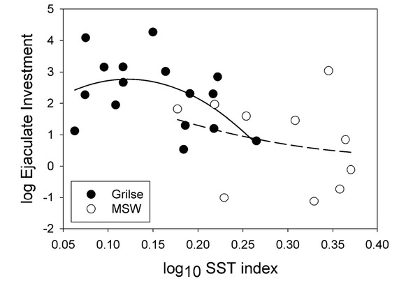
Figure 1
Polynomial form of the trade-off between primary and secondary sexual traits
ANCOVA, log Ejaculate investment in depending on log10 SST index with strategy (grilse vs multi-sea-winter) as a covariate. Grilse least square mean EI = 1.97, multi sea-winter least square mean EI = 1.31;
Model: r2 = 0.36, F = 6.345, p = 0.006
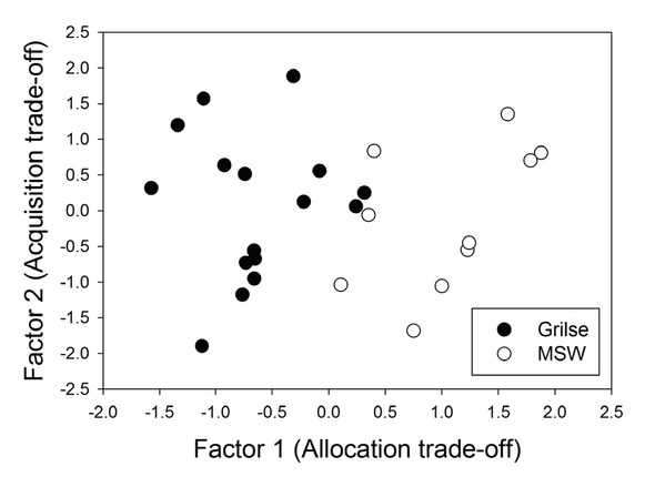
Figure 2
PC results for the correlation matrix of the four life history variables (sea age, smolt size, growth rate and log soma)
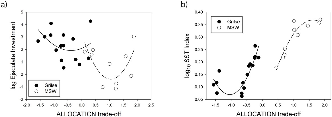
Figure 3
a. Polynomial function slopes depicting the effect of somatic condition/growth rate (ALLOCATION trade-off ) on ejaculate investment in grilse and anadromous adult males (see Table 2 for the components in the column PC1). ANCOVA reduced model, r2 = 0.301, F2,23 = 4.965, p = 0.016; within-cell regressions, strategy, F1,23 = 1.012, p> 0.05; SMOLT condition by fish age, F1,23 = 0.668, p > 0.05; b. Polynomial function slopes depicting the relationship between smolt size/growth rate on log10 SST investment in grilse and anadromous adult males (see Table 2 for the components in the column PC1). ANCOVA reduced model, r2 = 0.747, F2,23 = 33.90, p<0.001; within-cell regressions, strategy, F1,23 = 0.175, p> 0.05; SMOLT condition by fish age, F1,23 = 17.720, p < 0.01
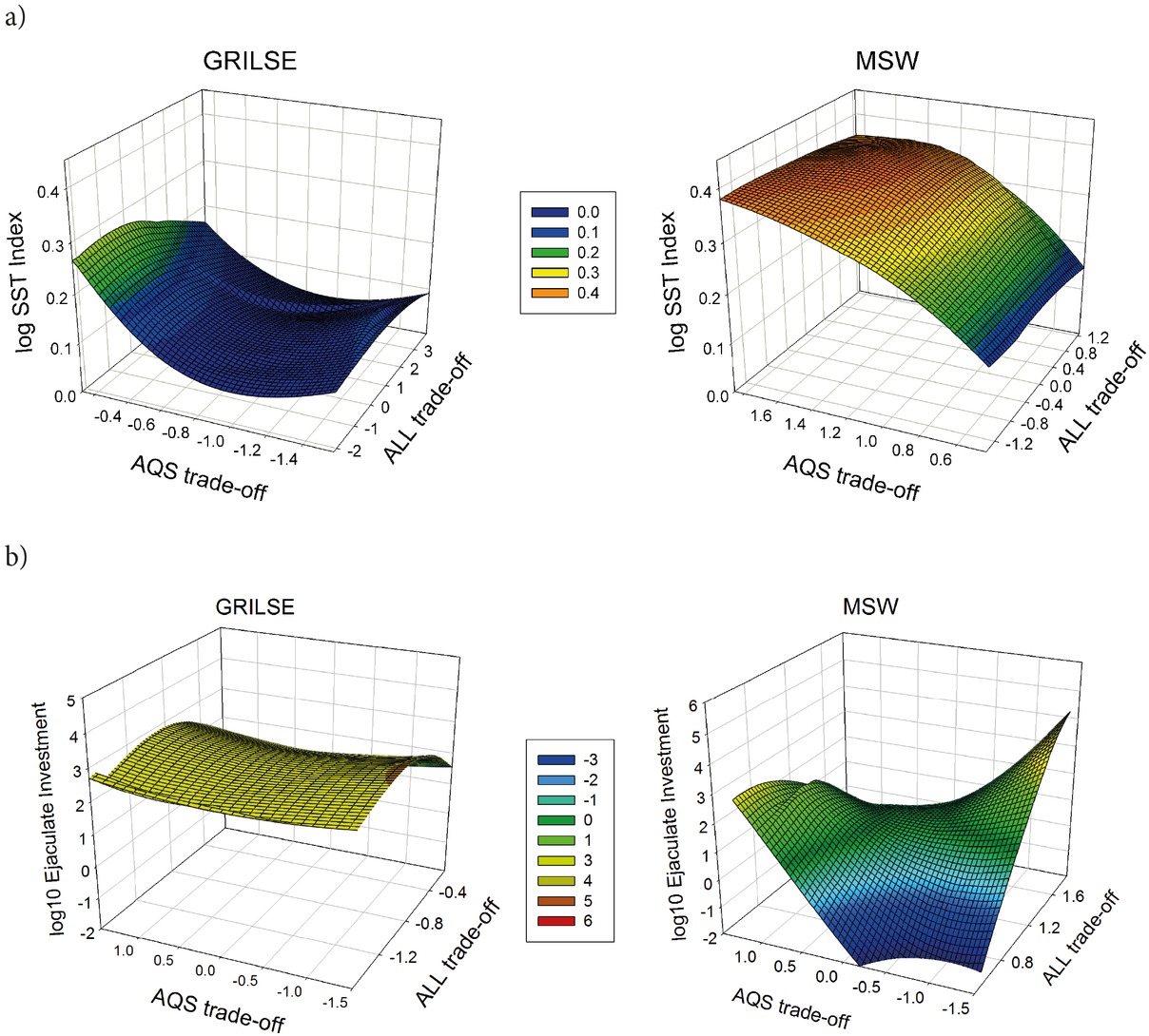
Figure 4
a. Model 1) The Model 1(M1) of the form of equation: y = a+b1×ALL+b2×AQS+c1×ALL2+c2×AQS2+d1×(ALL×AQS) assessed the amount of variation in SST (y) in relation to the allocation (ALL) and acquisition (AQS) trade-offs. Proportion of variance accounted for: 81%, R = 0.90 vs 0.57 for p=0.001 (Rolf and Sokal 2012; Table R); b. Model 2) The Model 2 (M2) of the form of equation: y = a+b1×ALL+b2×AQS+c1×ALL2+c2×AQS2+d1×(ALL×AQS) assessed the amount of variation in EI (y) in relation to the allocation (ALL) and acquisition (AQS) trade-offs. Proportion of variance accounted for: 51%, R = 0.71 vs 0.57 for p = 0.001 (Rolf & Sokal 2012; Table R)