
We examine the effects of compliance frictions in reclaiming foreign withholding taxes (WHTs) on Foreign Portfolio Investments (FPIs) and quantify their macroeconomic implications. Procedures for granting WHT refunds on cross-border investment are considered an important barrier to the free movement of capital that discourage cross-border investment and hinder the efficient allocation of capital via international financial markets. The return to portfolio investment in equity or debt securities made by a non-resident investor is typically subject to a WHT in the country of the investment (source country). To avoid double taxation, whenever the source WHT rate is higher than the reduced rate applicable according to the relevant double tax treaty, the non-resident investor can claim ex-post the refund of the excess—also “overwithheld” or “overpaid”—tax withheld by the source country. However, the current system for WHT refund in place in the EU proves cumbersome and costly, and prone to fraud.1
Lengthy and inefficient WHT refund procedures can give rise to three different sources of costs that can divert and/or discourage cross-border investment. First, claiming the refund entails direct financial costs arising from processing fees paid to the custodian or to an external service provider, paperwork, and diversity of source country requirements. Second, the delays—often years—in refunding investors bring about implicit financial losses for the investors and liquidity constraints, compared to the ideal scenario with immediate refund. Finally, the fact that some investors, particularly smaller ones, may decide to forego the refund for a number of reasons, makes the current system costly from a macroeconomic perspective, as it holds back cross-border investment. Overall, European Commission (2023) estimates these costs at EUR 6.62bn in 2022. By frustrating full integration of securities markets, these costs impede their functioning as the main channel of cross-border private risk sharing for firms and households.
Adding to the empirical literature on the effect of compliance costs (e.g., Pitt and Slemrod, 1989, and Benzarti, 2020), Jacob and Todtenhaupt (2023) estimate that FPI levels could be about 7.6% larger in the presence of a relief at source mechanism that eliminates most of the compliance costs in the reclaim process. Beyond the initial macroeconomic stimulus from the actual investment, enhanced FPI flows will impact the overall macroeconomic environment by raising total factor productivity and more generally, the efficiency of resource allocation in the recipient economy. In turn, this will have consequences for the main macroeconomic outcomes, such as GDP, the capital stock, and labor usage.
Beyond this background, we add to the quantification of the economic implications of lengthy and inefficient WHT relief procedures in two important ways. In a first step, we investigate the sensitivity of FPI stocks to overwithheld WHTs in the EU, separately for equity and debt holdings, and by type of holding investor (financial corporations, non-financial corporations, households, etc.). The analysis is based on a comprehensive panel of FPI stocks of 83 countries, including all EU member states, between 2005 and 2019 and country-pair specific WHT rates.
In line with the findings of Jacob and Todtenhaupt (2023), our analysis reveals a negative and statistically significant relationship between overwithheld WHTs and the stock of FPI in both equity and debt holdings. Specifically, our estimated elasticities suggest that a reduction of overwithheld WHTs by 1 percentage point is associated with a 1.5% increase in the stock of equity holdings in FPI. The effect on debt holdings is somewhat more modest but still significant, with an estimated increase of 0.7% for the same reduction in WHTs. At the sectoral level, the impact is consistently negative for financial corporations, while non-governmental investors other than financial firms, such as households, exhibit particularly pronounced negative effects on their equity holdings, possibly driven by the discouraging impact of tax complexities and the deterrent costs associated with reclaiming WHT overpayments.
In a second step, based on the econometric analysis, we are the first ones to quantify the macroeconomic impact of reducing the cost of WHT relief procedures making use of a general equilibrium model CORTAX (Bratta et al. 2023). The CORTAX model has been designed to simulate the economic impact of national and international tax policy reforms, as well as the international harmonization of national tax policies, taking into account the complex and multifaceted interactions between firms (including multinational enterprises (MNEs)), households, and governments.
The model results suggest that removing all frictions in the WHT refund procedures would lead to noticeable macroeconomic effects. On average across the EU27 countries, GDP is projected to increase by 0.26%, capital and wages would rise by 0.72% and 0.26%, respectively, and employment would increase marginally.
Typically, when individual investors receive dividends from foreign companies, they face taxation in both their home country and the country where the company is based, which includes a WHT. This tax treatment applies to both shares directly owned in foreign companies and those owned through pooled investment vehicles, such as mutual funds. Consequently, without any tax relief measures, these dividends are essentially subject to double taxation, with the remaining dividend after taxes being calculated as 1 minus the WHT of the source country minus the tax rate of the home country, multiplied by the dividend amount.
To prevent this double taxation, many countries offer a tax credit for the WHT paid in the foreign country against the taxes due domestically. With a tax credit, investors pay in their residence country only the residual tax due if the home country dividend tax rate is higher than the source country WHT, thus effectively avoiding double taxation. To allocate the taxing rights between the home country of the investor and the source country of the investment, numerous countries have entered into double taxation treaties (DTTs) that specify reduced WHT rates, typically between 10–15% under the model treaties of the Organization for Economic Cooperation and Development (OECD).
However, this system only works efficiently if investors can easily claim foreign tax credits. In practice, foreign countries might initially deduct taxes at their standard domestic rates, while the investor’s home country may only credit the reduced rate from the DTT. The difference between the higher taxes withheld by the foreign country and the lower tax credits allowed by the home country results in an excess WHT that investors must reclaim through a potentially complex process. We denote this difference the “Overwithheld WHT”.2
How might an investor obtain a refund for the overwithheld WHT? Central to the tax refund process is the “Residence certificate,” which serves as evidence to tax authorities abroad that the individual indeed resides in a different country. This certificate allows the tax officials in the source country to determine the appropriate amount of WHT refund based on the tax treaty with the investor’s country of residence.
Nonetheless, the source country may mandate various other formal documents and forms that the investor must procure before any tax refund is granted. Gathering, acquiring, and filling these documents can be a lengthy and sometimes expensive endeavor. In some cases, the costs in time and money to secure this tax relief can exceed the actual amount of WHT overpayment. We adopt the perspective of Slemrod and Sorum (1984) who define these expenses as compliance costs.
For the average retail investor, these compliance costs are typically prohibitive, resulting in a tendency not to pursue tax refunds at all. For example, a survey among 3,000 investors across the EU revealed that 70% of retail investors who experienced double taxation did not seek tax relief, citing the protracted and costly processes involved, leading some to even divest their foreign EU shares. About 30% of investors engage in the WHT reclaim process, of which less than half (46%) succeed in reclaiming WHT overpayments (Better Finance 2023).
Additionally, a 2021 survey by the European Central Bank indicated that WHT refund procedures within the EU were predominantly paper-based, requiring hard copies, physical signatures, and in-person interactions. The COVID-19 pandemic prompted some countries to test out more digital procedures for tax relief, occasionally permitting the use of electronic signatures and digital document submissions. While some EU Member States may offer digital alternatives for residence certificates, these are not always accepted by the tax authorities of the source country (European Central Bank 2023).
In essence, when investors do not seek reimbursement for overwithheld WHT, it reveals the lower bound of the cost of complying with tax regulations. This is because by choosing not to file for a tax refund, investors are opting to avoid the expenses related to compliance. As a result, the overwithheld WHT that is not claimed back becomes a real expense that diminishes the investor’s net returns. In other words, investors are effectively giving up the potential tax savings equivalent to the amount of the WHT overpayment because the costs of compliance are too burdensome. We follow prior studies on this topic (e.g., Benzarti (2020) and Jacob and Todtenhaupt (2023)) and interpret the tax deductions individuals or businesses do not claim as a measure of the costs involved in claiming them. Therefore, these unclaimed tax savings can be used as an approximation of the costs associated with tax compliance.3
The main source of data on FPI stocks is the “Coordinated Portfolio Investment Survey” (CPIS), conducted by the International Monetary Fund (IMF). Portfolio investment statistics report the international investment position of participating countries, that is their holdings of portfolio investment assets in the form of equity and investment fund shares, long-term debt securities (i.e., debt securities with an original maturity over one year), and short-term debt securities (i.e., debt securities with an original maturity of one year or less). The statistics are reported on an annual basis and are broken down by counterpart economies (those whose residents have issued the securities).4,5
Separate reporting of debt and equity holding allows one to analyze the behavior of the two series separately. Likewise, the CPIS data cover cross-border positions in equity and debt securities, disaggregated by sector of the holder. These are (1) the central bank, (2) deposit-taking corporations except the central bank, e.g. commercial and savings banks, (3) other financial corporations, e.g. insurance, pension, and money market funds, (4) general government except the central bank, and (5) the group of non-financial corporations, households, and non-profit institutions serving households (NPISHs).6,7,8
We restrict our sample to the 27 member states of the EU as issuers of equity and debt securities. On the investor side, our sample comprises 81 and 83 countries in the case of equity and debt securities, respectively. All available country-pairs and the number of observations for each specific case are shown in Tables A.3 and A.4 in the Appendix for the case of total equity and total debt FPI stocks, respectively. In both cases, more than half of all country-pairs have at least 13 country-pair-year observations, which gives an indication of the balanced nature of the data.
Table 1 below provides descriptive statistics for the stock of bilateral equity and debt securities holdings. The average total equity FPI of an investor country in a particular issuer country in our sample is $4.3 billion. It is $6.0 billion in the case of debt FPI. At the sectoral level, “Other Financial Corporations” and “Households” hold relatively large stocks of equity on average, while the average equity stocks of the “Central Bank” and “NPISHs” are relatively small. Similarly, in the case of debt securities, we observe comparably large positions among “Other Financial Corporations” and “Depository-taking Corporations”, while the other sectors hold relatively small positions on average.
Descriptive statistics of bilateral FPI stocks
| Obs. | Mean | Std. Dev. | Min. | Median | Max. | |
|---|---|---|---|---|---|---|
| Total bilateral equity FPI (mio. Dollar) | 22,302 | 4,256.6 | 25,062.5 | 0 | 14.8 | 697,804.7 |
| (1) Central Bank | 8,687 | 17.6 | 260.9 | 0 | 0 | 8,553.6 |
| (2) Depository-taking Corporations | 13,318 | 194.9 | 1,173 | 0 | 0 | 25,822.1 |
| (3) Other Financial Corporations | 15,375 | 2,596.9 | 16,923.4 | 0 | 5.9 | 438,339 |
| (4) General Government | 11,320 | 194.3 | 1,484.8 | 0 | 0 | 43,860.9 |
| (5a) Nonfinancial Corporations | 10,319 | 244.8 | 2,480.1 | 0 | 0 | 110,203 |
| (5b) Households | 9,805 | 1,019.4 | 11,893.5 | 0 | 0.2 | 317,544.7 |
| (5c) NPISHs | 7,391 | 40.5 | 348.4 | 0 | 0 | 11,247.5 |
| Total bilateral debt FPI (mio. Dollar) | 23,079 | 6,012 | 24,300.6 | 0 | 57.6 | 343,959.2 |
| (1) Central Bank | 10,452 | 354.8 | 2,345.1 | 0 | 0 | 71,254.7 |
| (2) Depository-taking Corporations | 16,420 | 1766 | 8446 | 0 | 4 | 176,231 |
| (3) Other Financial Corporations | 16,081 | 3,462.9 | 15,655.3 | 0 | 14.9 | 238,400.9 |
| (4) General Government | 13,554 | 244.3 | 1,695.1 | 0 | 0 | 45,884.8 |
| (5a) Nonfinancial Corporations | 11,391 | 127.1 | 891.7 | 0 | 0 | 27,860 |
| (5b) Households | 10,871 | 178.9 | 1,345.8 | 0 | 0.1 | 3,3468 |
| (5c) NPISHs | 8,833 | 28.7 | 206.2 | 0 | 0 | 4,968.9 |
Source: CPIS.
Data on WHTs and tax treaties come primarily from country specific WHT tables sourced from the International Bureau of Fiscal Documentation (IBFD). Using these data, we identified the relevant WHT rates applicable to dividends and negotiable (i.e. tradeable) debt securities.
The average “Overwithheld WHT” on equity is shown in Panel A of Figure 1, separately for each group of residence countries. On average, it fluctuates between values of five to eight percentage points, with those for residence countries in Oceania marginally larger than those in Africa, the Americas, Asia, and Europe. Similarly, as can be seen from Panel B, the “Overwithheld WHT” on debt securities is lying within a range of four to eight percentage points, with those for residence countries in Europe larger than the other residence countries, at least until 2016. Figure 2 displays the number of country-pair specific bilateral tax treaties in place in our sample, gradually rising from 1,286 in 2005 to 1,540 in 2019.9
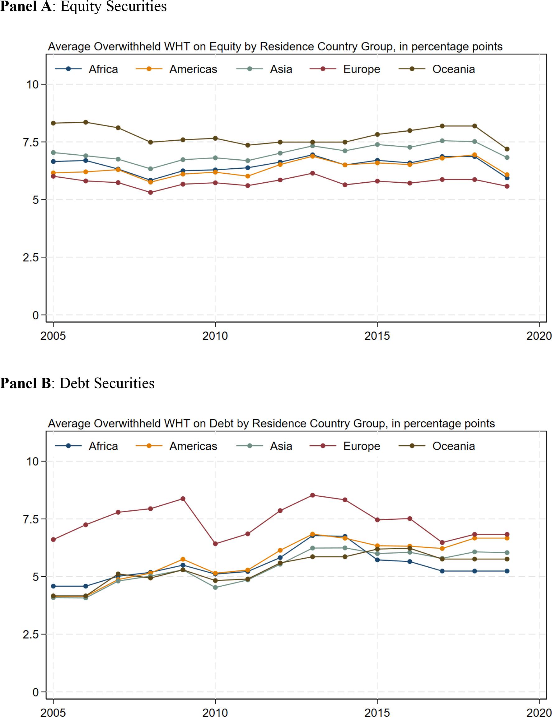
Average overwithheld WHT on equity and debt by residence country group.
Notes: Panel A displays the average “Overwithheld WHT” on dividends for individual investors, by group of residence country. Similarly, Panel B displays the average “Overwithheld WHT” on tradable debt for individual investors, by group of residence country.
Source: IBFD and authors’ calculations.
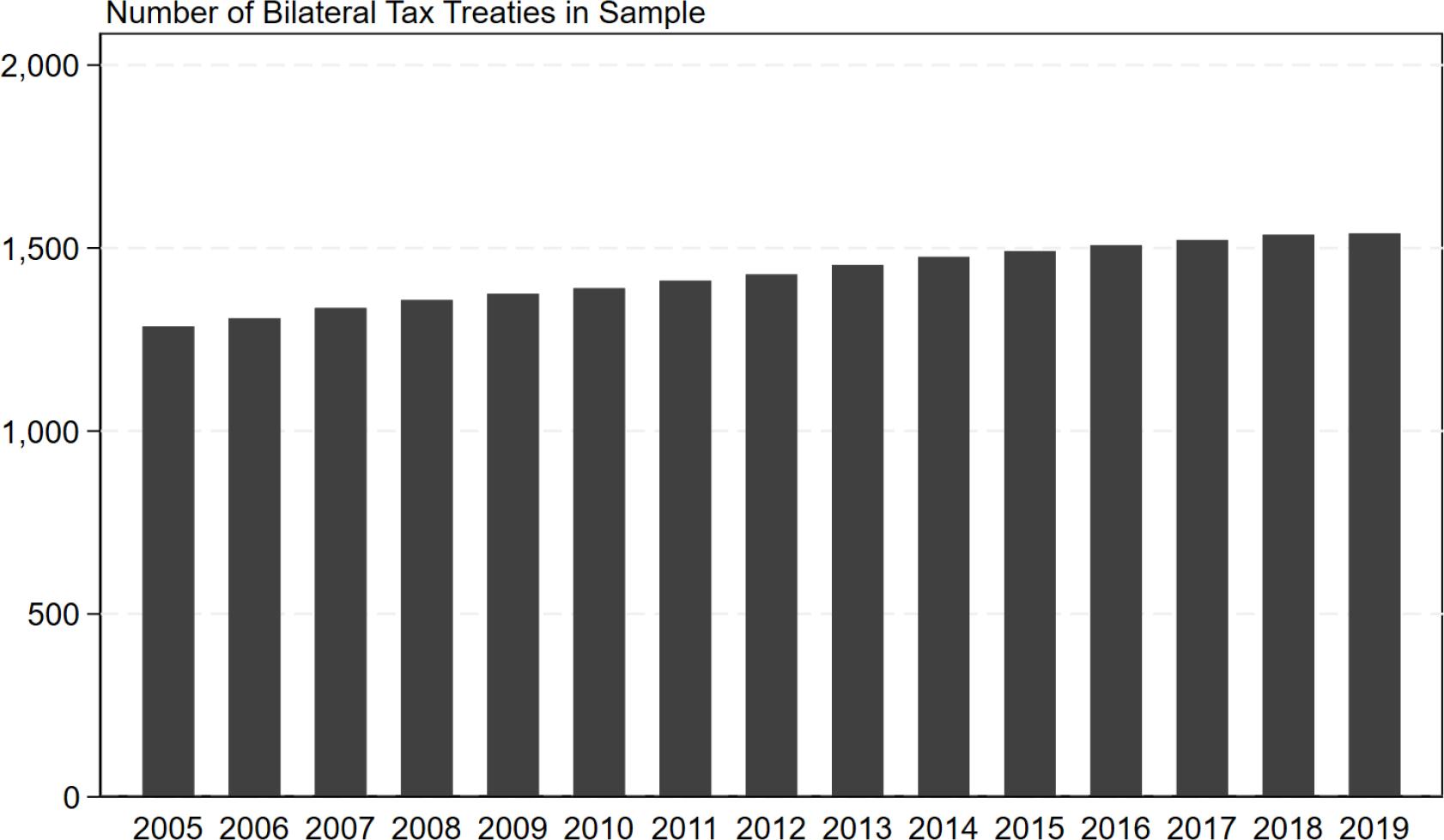
Number of bilateral tax treaties in sample data.
Notes: The figure shows the total number of bilateral tax treaties in place in our sample.
Source: IBFD and authors’ calculations.
Figure 3 provides an initial visual representation of the empirical relationship, plotting the amount of “Overwithheld WHT” against the stock of FPI in equity and debt. Panel A of the figure uses the horizontal axis to represent the “Overwithheld WHT” and the vertical axis to show the total FPI stock of equity holdings, while Panel B does the same for the FPI stock of debt securities. A cursory inspection of the data reveals a noticeable and consistent negative correlation, where higher amounts of “Overwithheld WHT” tend to be associated with lower FPI amounts.
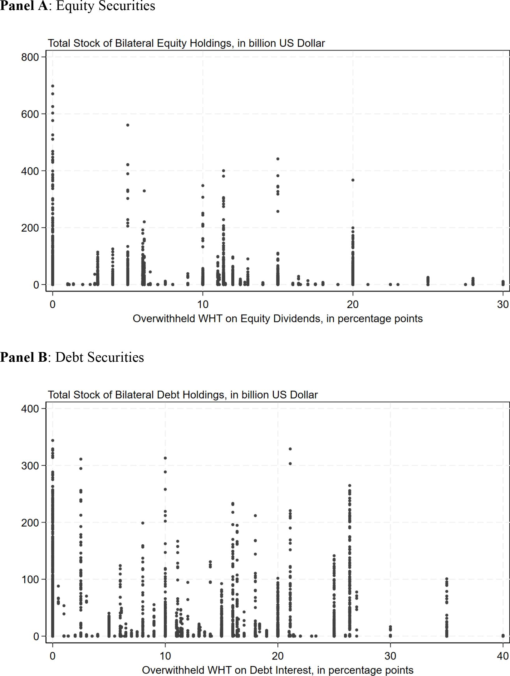
Relationship between Equity and Debt FPI and “Overwithheld WHT”.
Notes: Panel A is plotting the total stock of bilateral equity holdings on the vertical axis against “Overwithheld WHT” on equity holdings on the horizontal axis. Similarly, Panel B is plotting the total stock of bilateral debt holdings on the vertical axis against “Overwithheld WHT” on debt holdings on the horizontal axis.
Source: IBFD and CPIS.
When examining the data and the nature of our dependent variable, FPI stocks, we find two noteworthy patterns that eventually influence our choice of modelling approach. First, a significant number of observations for the dependent variable are zeros: 4,747 instances (21.3% of the sample) for equity and 4,197 (18.2% of the sample) for debt. Second, a clear pattern of heteroskedasticity is observed, where larger overpayments of WHT corresponding to smaller variances in the FPI stocks of equity and debt. Thus, estimating the semi-elasticity of the stock of FPI with respect to “Overwithheld WHT” using a log-linearized model and ordinary least squares (OLS) would encounter two significant problems. The first problem arises from the handling of zero bilateral FPI values in log-linearized models, and the second is a potential bias due to Jensen’s inequality.
To address the first issue, two solutions could be thought of: using only non-zero FPI observations in the estimation or adding a constant (such as 1) to the FPI stocks to avoid taking the logarithm of zero. However, excluding zero values could result in a significant loss of information, while artificially adjusting the FPI stocks could lead to biased estimations due to model misspecification.
The second problem pertains to the bias introduced by Jensen’s inequality, which states that the expected value of the logarithm of a random variable does not equal the logarithm of its expected value and is influenced by the variable’s mean and variance. If the variance of the error term in the model correlates with the independent variables, as the evidence in Figure 3 suggests, this would lead to biased estimations.
To overcome these challenges, we opt for the Poisson pseudo-maximum-likelihood (PPML) method, which allows us to estimate the dependent variable in its raw form rather than as log values. This technique, as demonstrated in Santos Silva and Tenreyro (2006), is robust against various heteroskedasticity patterns and addresses the issue of Jensen’s inequality without requiring logarithmic transformations, thus preserving the original sample structure.10,11
In particular, the following baseline specification is estimated:
Where FPIim,t is the stock of FPI from home (investor) country i in EU member state (source) m in year t; OverwithheldWHTmi,t is a time-variant vector of “Overwithheld WHT” in member state m towards an investor from country i; μit, θmt and γim are, respectively, vectors of home-year, source-year, and time-invariant country-pair fixed effects. A unit increase in a covariate will lead to a 100 × (eβ – 1) percentage increase in the FPI stock.
The rich fixed-effects structure is complemented by a set of covariates, βXim,t, that vary over time at the country-pair level, mirroring financial and economic dynamics. We are closely following Jacob and Todtenhaupt (2023) and control for the presence of a bilateral tax treaty to account for the fact that WHT overpayments are zero if there is no treaty in force. We further control for the bilateral exchange rate, differences in the overall and per capita GDP growth, the relative difference in domestic credit supply to the private sector, and the relative difference in domestic credits by banks.12
The rich structure of fixed effects and time-variant country-pair covariates allows for the isolation of the effects of “Overwithheld WHT” on FPI from within country-pair variation over time. Specifically, home-year and source-year fixed effects control for any countryyear specific institutional, economic, legal, or other changes in either country that may affect cross-border investment, such as GDP, GDP per capita, (financial) market attractiveness, access to financial markets, or changes in corporate taxes and tax enforcement. Timeinvariant country-pair fixed effects account for any covariates that are specific (and constant) for a given pair of countries over time, including geographical distance, common language, and past colonial relationship. To put it differently, the coefficient β1 is identified only from bilateral within-country-pair variation in “Overwithheld WHT” over time.
One concern in our setup is the potential endogeneity of overwithheld WHT with respect to economic conditions and policy measures that could in turn affect FPI stocks. Table 2 reports the Pearson correlation coefficients of country-pair level changes in equity and debt WHT overpayments with various economic variables at the country-pair level. Reassuringly, we find that neither changes in overwithheld WHT on equity nor debt are directly correlated with any of these, with the exception of whether a bilateral tax treaty is in place and differences in GDP per capita growth rates. Given the set of fixed effects and additional covariates at the country-pair level, this provides some assurance of the validity of our empirical approach. Nevertheless, we cannot fully rule out the existence of other timevarying country-pair level determinants of FPI stocks that we do not control for.13
Descriptive statistics of bilateral data: Correlation matrix
| [1] | [2] | [3] | [4] | [5] | [6] | [7] | [8] | |
|---|---|---|---|---|---|---|---|---|
| [1] Y-o-Y changes in Overwithheld WHTs (equity) | 1 | |||||||
| [2] Y-o-Y changes in Overwithheld WHTs (debt) | 0.1733 | 1 | ||||||
| [3] Dummy: DTT in placeiim,t | 0.0160 | 0.0208 | 1 | |||||
| [4] Rel. diff. in exchange ratesim,t | 0.0060 | 0.0083 | –0.0674 | 1 | ||||
| [5] Rel. diff. in GDP growthim,t | -0.0042 | 0.0016 | –0.0059 | 0.0008 | 1 | |||
| [6] Rel. diff. in GDP (p.c.) growthim,t | –0.0152 | –0.0041 | 0.0344 | –0.0487 | 0.0161 | 1 | ||
| [7] Rel. diff. in domestic credit to the private sectorim,t | 0.0099 | –0.0007 | –0.1609 | 0.0925 | –0.0010 | –0.0421 | 1 | |
| [8] Rel. diff. in domestic credit by banksim,t | 0.0077 | 0.0004 | –0.1578 | 0.1111 | 0.0000 | –0.0387 | 0.9842 | 1 |
Notes: The table reports the Pearson correlations between the individual regression covariates. Correlations which are significant at the 10% level are indicated in bold. Details on the computation and the source of each variable can be found in Table A.1 in the Appendix.
The main results on the effects of overwithheld WHT on the total stock of equity and debt holdings are presented in Tables 3 and 4, respectively. In general, the estimation results indicate a negative and statistically significant elasticity of the FPI stock of equity and debt holdings to “Overwithheld WHT”. Concretely, starting with the case of no additional covariates (column 1), the estimated semi-elasticity implies that a one percentage point reduction in overwithheld WHT increases the FPI stock of equity holdings by about 1.5%.14 Reassuringly, the results from the fixed-effects specifications hold up to the inclusion of covariates in columns 2 to 4, with only marginal changes to the estimated impact from “Overwithheld WHT”.15
Effects of overwithheld WHT on equity FPI holdings
| (1) | (2) | (3) | (4) | |
|---|---|---|---|---|
| OverwithheldWHTmi,t | –0.0151*** (0.008) | –0.0162*** (0.004) | –0.0162*** (0.004) | –0.0168*** (0.008) |
| Dummy: DTT in placeim,t | 0.0182 (0.914) | 0.0172 (0.919) | –0.0034 (0.985) | |
| Rel. diff. in exchange ratesim,t | –0.0010 (0.244) | –0.0010 (0.243) | –0.0011 (0.198) | |
| Rel. diff. in GDP growthim,t | 0.0001* (0.094) | 0.0001* (0.097) | ||
| Rel. diff. in GDP (p.c.) growthim,t | –0.0000 (0.864) | –0.0000 (0.956) | ||
| Rel. diff. in domestic credit to the private sectorim,t | 0.0910 (0.508) | |||
| Rel. diff. in domestic credit by banksim,t | –0.3534*** (0.000) | |||
| No. of obs. | 22,302 | 21,477 | 21,237 | 18,581 |
| Pseudo R2 | 0.9937 | 0.9941 | 0.9941 | 0.9946 |
| Home-year FE | YES | YES | YES | YES |
| Source-year FE | YES | YES | YES | YES |
| Country-pair FE | YES | YES | YES | YES |
Notes: Estimated coefficients from the Poisson pseudo-maximum-likelihood (PPML) method. The dependent variable in all columns is the stock of equity FPI holdings in country i of investors residing in country m in year t.
indicate significance at the 1%, 5%, and 10% levels, respectively. Standard errors clustered by country-pair level. Corresponding p-values are shown in brackets below each coefficient estimate. The coefficient estimate of the intercept is omitted to ease readability.
Effects of overwithheld WHT on debt FPI holdings
| (1) | (2) | (3) | (4) | |
|---|---|---|---|---|
| OverwithheldWHTmi,t | –0.0073** (0.039) | –0.0065* (0.074) | –0.0065* (0.072) | –0.0071* (0.059) |
| Dummy: DTT in placeim,t | –0.1199 (0.389) | 0.1197 (0.389) | –0.1217 (0.407) | |
| Rel. diff. in exchange ratesim,t | –0.0002 (0.677) | –0.0003 (0.665) | –0.0003 (0.590) | |
| Rel. diff. in GDP growthim,t | 0.0000 (0.654) | 0.0000 (0.833) | ||
| Rel. diff. in GDP (p.c.) growthim,t | –0.0012*** (0.000) | –0.0013*** (0.000) | ||
| Rel. diff. in domestic credit to the private sectorim,t | 0.3781** (0.016) | |||
| Rel. diff. in domestic credit by banksim,t | –0.4180*** (0.001) | |||
| No. of obs. | 23,079 | 22,275 | 22,012 | 19,111 |
| Pseudo R2 | 0.9859 | 0.9863 | 0.9864 | 0.9865 |
| Home-year FE | YES | YES | YES | YES |
| Source-year FE | YES | YES | YES | YES |
| Country-pair FE | YES | YES | YES | YES |
Notes: Estimated coefficients from the Poisson pseudo-maximum-likelihood (PPML) method. The dependent variable in all columns is the stock of debt FPI holdings in country i of investors residing in country m in year t.
indicate significance at the 1%, 5%, and 10% levels, respectively. Standard errors clustered by country-pair level. Corresponding p-values are shown in brackets below each coefficient estimate. The coefficient estimate of the intercept is omitted to ease readability.
The corresponding effect on FPI stock of debt holdings is slightly smaller in magnitude, estimated between –0.1% and 1.4% (point estimate 0.7%) for a one percentage point reduction in “Overwithheld WHT” (Column 1 in Table 4). As before, further controlling for the presence of a bilateral tax treaty, the relative difference in the exchange rate, differences in the overall and per capita GDP growth rates, the difference in domestic credit supply to the private sector, and the difference in domestic credits by banks does not significantly alter the coefficient estimate.
Our sectoral analysis differentiates between financial corporations including depository-taking and other financial institutions, and other non-governmental investors, including non-financial corporations, households, and NPISHs. A priori, we posit that the impact of “Overwithheld WHT” on investment stocks may vary between these groups due to factors such as the specialized tax expertise and resources of financial corporations, their ability to achieve economies of scale in the tax reclaim process, and the higher frequency of their investment transactions. These factors likely affect their propensity to engage in and benefit from tax recovery efforts. In contrast, other investors might perceive the refund process as too complex or costly relative to the potential benefits, particularly when investment transactions occur less frequently. The motivation to optimize tax efficiency is also presumably more acute for financial corporations, whose bottom lines and market competitiveness are directly affected.
Table 5 presents the impact of “Overwithheld WHT” on equity FPI holdings across different investor groups, focusing on a subset of data points where equity stock information is available for all groups, due to the more limited CPIS data at a granular level. The first column, which shows the effect on the total equity stock, serves as a reference for assessing the disaggregated effects. The influence of “Overwithheld WHTs” is slightly smaller when compared to the full sample analysis (refer to column 3 of Table 3). Disaggregated results reveal that non-financial corporations, households, and NPISHs experience an impact substantially larger in size and above average from “Overwithheld WHT” on their equity holdings than financial corporations do.16 Turning to the impact on investors’ FPI in debt securities shown in Table 6, the results point towards stronger effects among financial corporations. We do not find any effects among other investors, possibly related to the fact that their debt holdings are comparably small on average.
Sectoral effects of overwithheld WHT on equity FPI holdings
| (1) All investors | (2) Financial institutions | (3) Other investors (NFC, HH, NPISHs) | |
|---|---|---|---|
| OverwithheldWHTmi,t | –0.0131* (0.087) | –0.0104* (0.088) | –0.0255* (0.068) |
| Dummy: DTT in placeim,t | 0.4052 (0.128) | 0.2479 (0.246) | 0.9414** (0.025) |
| Rel. diff. in exchange ratesim,t | –0.0006 (0.608) | 0.0016 (0.538) | –0.0036 (0.240) |
| Rel. diff. in GDP growthim,t | 0.0001 (0.190) | 0.0001 (0.143) | 0.0000 (0.573) |
| Rel. diff. in GDP (p.c.) growthim,t | –0.0009 (0.206) | –0.0012* (0.079) | –0.0003 (0.691) |
| No. of obs. | 10,244 | 10,244 | 10,244 |
| Pseudo R2 | 0.9965 | 0.9962 | 0.9948 |
| Home-year FE | YES | YES | YES |
| Source-year FE | YES | YES | YES |
| Country-pair FE | YES | YES | YES |
Notes: Estimated coefficients from the Poisson pseudo-maximum-likelihood (PPML) method. The dependent variable in each column is the stock of equity FPI holdings in country i of investors residing in country m in year t by type of investor.
indicate significance at the 1%, 5%, and 10% levels, respectively. Standard errors clustered by country-pair level. Corresponding p-values are shown in brackets below each coefficient estimate. The coefficient estimate of the intercept is omitted to ease readability.
Sectoral effects of overwithheld WHT on debt FPI holdings
| (1) All investors | (2) Financial institutions | (3) Other investors (NFC, HH, NPISHs) | |
|---|---|---|---|
| OverwithheldWHTmi,t | –0.0114** (0.049) | –0.0147*** (0.008) | 0.0016 (0.810) |
| Dummy: DTT in placeim,t | 0.1634 (0.272) | 0.2297 (0.172) | –0.6556 (0.318) |
| Rel. diff. in exchange ratesim,t | –0.0007 (0.283) | –0.0018** (0.040) | 0.0007 (0.671) |
| Rel. diff. in GDP growthim,t | 0.0000 (0.827) | 0.0001 (0.474) | –0.0005** (0.043) |
| Rel. diff. in GDP (p.c.) growthim,t | –0.0003 (0.649) | –0.0008 (0.134) | 0.0068 (0.128) |
| No. of obs. | 12,021 | 12,021 | 12,021 |
| Pseudo R2 | 0.9874 | 0.9874 | 0.9746 |
| Home-year FE | YES | YES | YES |
| Source-year FE | YES | YES | YES |
| Country-pair FE | YES | YES | YES |
Notes: Estimated coefficients from the Poisson pseudo-maximum-likelihood (PPML) method. The dependent variable in each column is the stock of debt FPI holdings in country i of investors residing in country m in year t by type of investor.
indicate significance at the 1%, 5%, and 10% levels, respectively. Standard errors clustered by country-pair level. Corresponding p-values are shown in brackets below each coefficient estimate. The coefficient estimate of the intercept is omitted to ease readability.
The results are corroborated by several robustness tests. First, a bias correction procedure for PPML models with two- and three-way fixed effects is applied.17 Table A.2 in the Appendix presents both the original estimates from the baseline estimations (as shown in column 1 of Tables 3 and 4) and the results obtained using the bias-corrected methodology. While the magnitude of the coefficient estimates and their associated standard errors are slightly larger with the bias correction, the differences are marginal.
In addition, the baseline model is estimated on interval data, keeping only every third or every fourth year from our panel in order to rule out time-period specific effects.18 The main results on the total FPI stock of equity and debt holdings remain unchanged.19
The second part of the analysis is concerned with the macroeconomic impact of reducing the cost of WHT refund procedures, based on the computable general equilibrium model CORTAX. CORTAX is designed to simulate the economic impact of national and international corporate tax policy reforms, as well as the international harmonization of national tax policies. It is capable of accounting for the complex and multifaceted interactions between domestic and multinational firms, households, and governments. CORTAX is a multicountry model with a full calibration for 30 countries, namely each of the EU27 member states, the UK, the US, and Japan. Additionally, there is a notional tax haven, to which a proportion of profits can be shifted. It has been used extensively in both academic and policy contexts. A short overview of its main buildings blocks and their links is provided here, with more details of the model characteristics and its parameterization given in Bratta et al. (2023).
Being a macroeconomic model, CORTAX models aggregate economic variables, such as GDP, investment, consumption, employment, and fiscal revenue, and captures linkages between firms, households, and governments. The special features of CORTAX are those designed to capture aspects of corporate income taxation, such as multinational profit shifting, investment decisions, loss compensation, and debt-and- equity financing. Countries are linked to each other via international trade in goods markets, investment by MNEs, international capital flows, and intermediate inputs within MNEs.
In order to capture important aspects of the corporate tax system, CORTAX divides firms into three categories: MNE headquarters, MNE subsidiaries in each of the other countries, and domestic firms that only operate in their home country. Each country has one representative domestic firm and one MNE headquarter. This MNE headquarter owns a representative MNE subsidiary in each of the other countries. All firms produce output using the factors of production, namely labor, capital, and a location-specific fixed factor. MNE subsidiaries additionally use an intermediate good from its MNE headquarter. Domestic firms maximize own profits, while MNEs maximize the global profits of the headquarter and all subsidiaries combined, including any benefits from engaging in profit shifting.
Households in CORTAX maximize their lifetime utility subject to their lifetime budget constraint. They live for two generations: young (age 20–59) and old (age 60–99). Households receive utility from consumption and disutility from working. Young households choose their levels of work, consumption, and savings to maximize their inter-temporal utility.
The model solves to a general equilibrium, meaning that households and firms adjust their behavior to maximize their welfare given the exogenous conditions and the optimal behavior of the other agents. This implies that the goods market clears, and the factor markets for both labor and capital clear, through adjustments in the quantities of labor and capital and the wage rate. In the asset market, which also clears, bonds and equities are partially substitutable from the perspective of households’ savings portfolios. Bonds and equities of different origins are freely traded across borders. Therefore, the gross rates of return to these assets are fixed at the world level. The current account equals the trade balance plus net foreign earnings. Governments in CORTAX perform the functions of collecting tax revenue, spending on government consumption, providing transfers to households, and servicing public debt. Furthermore, the government budget must be balanced by adjusting revenues or expenditures.
A notable feature of CORTAX is the modelling of profit shifting. First, this is modelled as transfer pricing that occurs between multinational headquarters and their associated subsidiaries. Second, the model allows firms to shift part of their tax base to a tax haven. This is modelled as a separate channel for profit shifting than transfer pricing between MNE headquarters and subsidiaries.
Simulations are implemented either by changing exogenous parameters (such as in this exercise) or by changing the system of equations (such as when simulating a consolidation of the MNE corporate tax base) and re-solving the model. CORTAX computes the long-run general equilibrium, reflecting complete behavioral adjustments by households and firms to the new economic conditions, such as improved crossborder investment incentives. This includes reallocation of capital and subsequent shifts in employment demand, wages, savings, corporate profits, tax revenues, etc. To arrive at this new steady state, firms and households fully adjust their behavior to optimize their profits and welfare, given the new conditions and the optimizing behavior of other economic agents.
The simulations are run using a small-open economy assumption, which we believe to be most appropriate for EU countries, especially in the long run. This is relevant because the gross return to capital is principally determined in world capital markets (though country differences persist due to source taxes). Therefore, when the net return on investment increases, as it does in our simulation, the equilibrium amount of capital is expected to rise in the long run.20
While WHTs and related administrative costs from reclaiming overpayments are not explicitly modelled in CORTAX, they are reflected by adjusting the taxdeductibility of the administrative cost related to investments abroad, thereby ultimately reducing the effective costs of foreign investments. Concretely, the model includes a cost of financial distress, which may be different across multinational firms in each of the countries where their subsidiaries are present. This cost may be directly deductible from each of the CIT base paid by every subsidiary. For example, the relevant parameter, which is denoted by βc, will be zero or one if either no or full deductibility is allowed, respectively. In principle, it can also take larger values than one. While in the baseline of the model, the deductibility of this cost is set to zero, the concrete reform at hand is simulated by allowing a positive value of the deductibility parameter, thereby effectively decreasing the costs related to investments abroad and, therefore, the marginal cost of financing. Ceteris paribus, this leads to an increase in the net return on foreign investments and strengthens incentives to invest abroad.
Following established methods in the empirical trade literature, so-called ad valorem equivalents (AVEs) are computed. Economists frequently use AVEs, also called “tariff equivalents”, as a shorthand to capture the price and quantity effects of non-tariff barriers (NTB) to trade, such as quotas, subsidies, customs delays, technical barriers, or other systems preventing or impeding trade flows. Following the quantity-approach laid out in Kee et al. (2009), AVEs are computed as the equivalent tariff that would be necessary to obtain the same proportionate change in quantity traded due to the presence of NTBs.
Concretely, the computation of AVEs follows in two steps. First, one needs to determine the proportionate change in the quantity of trade that is due to the presence of NTBs, e.g. from gravity-type models. Then, in a second step, one uses the elasticity of trade with respect to a one percentage point increase in the tariff to convert the proportionate change in quantity imported due to NTBs in terms of AVEs.21
In this case, the equivalent deductibility that could rationalize the change in FPI, taking the semi-elasticity of foreign investments with respect to the deductibility within CORTAX (η
The numerator of Eq. (1), the percentage change in FPI, requires two ingredients: the actual level of FPI and the hypothetical level of FPI in the absence of any costs from WHT relief procedures. While the former can be directly observed in the data (e.g., how much do investors from the United States invest in Italy in a given year under the status quo), the latter must be inferred from estimated regressions by using predicted values of FPI levels with no costs from WHT overpayment.
The semi-elasticity of –1.5 is directly obtained from the empirical analysis above (see column 1 of Table 3) to compute hypothetical levels of foreign equity portfolio investments in the absence of any WHT complexities,
The denominator of Eq. (1), the tax semi-elasticity within CORTAX, ηCORTAX, can be easily obtained from “within” the model by increasing the deductibility by one percentage point and observing the resulting change in foreign investments. The average semielasticity of investments is found to be 2.79, i.e., increasing the tax deductibility by one percentage point leads to an increase in foreign investments by around 2.79%. The semi-elasticity exhibits some degree of crosscountry heterogeneity, reflecting differences in the value of the tax deductibility. For example, it features a positive correlation with the domestic effective CIT rate.22
As a final step, the corresponding values for the deductibility-equivalent are easily derived by applying Eq. (1) from above: by how much would the deductibility need to increase in CORTAX in order to replicate a change in foreign investments of the same magnitude that the first part of the analysis has suggested, taking as a given the elasticity of foreign investments with respect to the deductibility. We use observations from the most recent year in the sample, 2019, and those country-pairs, which are modelled in CORTAX.23 When computing the median value across all remaining observations a value of 2.14 is obtained to be used as the change in deductibility, βc.24 This shock is applied to all EU countries.
Given that FPI is not explicitly modelled in CORTAX, in this exercise it is assumed that FPI and FDI (foreign direct investment, which is explicitly modelled) have similar macroeconomic consequences in the long run. Put simply, what we aim to capture is increased cross-border ownership of capital. Key distinctions between FPI and FDI are the degree of liquidity and the extent of foreign control. However, as we are concerned with long run stock positions and representative foreign investors, these distinctions are not salient to the analysis. The reduction of “Overwithheld WHT” can be expected to boost the foreign-owned capital available within the destination countries, and this is what is represented in our simulations. Beyond this background, no assumption is made concerning the average for the EU27 as a whole. Nonetheless, to the extent to which in a given country stock positions of FPI vary from those of FDI, this could impact the magnitude of the effects for those countries.25
The model’s results suggest that eliminating all frictions in the WHT refund procedures would, on average, result in gains for all major economic indicators across the EU27 countries. In the baseline scenario, the EU’s GDP is projected to increase by 0.26%, which is equivalent to EUR 46 billion in nominal 2024 terms. The capital stock of the EU is expected to experience the most significant growth, with an estimated rise of about 0.7%. Additionally, wages are projected to increase by 0.26%, and employment is anticipated to see a marginal rise of 0.07% relative to the current situation. The projected impact on the EU’s GDP is considerably larger than previous static estimates, such as the approximately EUR 7 billion forecasted by the European Commission (2023), highlighting the dynamic, growthenhancing effects of increased investment in a general equilibrium context.
Although the CORTAX macroeconomic model does not provide explicit uncertainty measures for its forecasts, we leverage the confidence intervals around the empirical semi-elasticity point estimate to calculate a lower bound of the potential macroeconomic impact. By applying the lower limit of the semi-elasticity derived from our baseline analysis (as shown in column 1 of Table 3 and referenced in footnote 14), we arrive at a conservative assessment of the equivalent tax deduction, βc. While this lower-bound estimate is more modest, the removal of overwithheld WHT would still yield substantial benefits for the EU’s GDP—nearly EUR 8 billion—alongside positive effects on capital stock, wages, and employment.
This study examines the economic implications of compliance frictions associated with the refund procedures of overwithheld WHT, which have shown to be a lengthy and burdensome process for international investors. In line with previous results, we find that these costs discourage investors from investing abroad. We find a negative and statistically significant elasticity of the FPI stock of equity and debt holdings to overwithheld WHT. Concretely, the estimated elasticities imply that a one percentage point reduction in overwithheld WHT increases the FPI stock of equity holdings by 1.5%. The effect on debt holdings is somewhat smaller but still significant, with an estimated increase of 0.7% for the same reduction in “Overwithheld WHT”. At the sectoral level, the impact is consistently negative for financial corporations, while non-governmental investors other than financial firms, such as households, exhibit particularly pronounced negative effects on their equity holdings, possibly driven by the discouraging impact of tax complexities and the deterrent costs associated with reclaiming WHT overpayments.
The macroeconomic effects of such frictions are non-negligible. Based on a comprehensive general equilibrium model, we find that eliminating compliance costs for investors could increase EU GDP by 0.26%, equivalent to EUR 46 billion in nominal 2024 terms, alongside positive effects on capital stock, wages, and employment.