
Table 1
The chemical composition of 9XC steel.
| Chemical composition, wt.% | |||||||||
|---|---|---|---|---|---|---|---|---|---|
| C | Si | Mn | Cr | Mo | Al | Ni | P | S | V |
| 0.94 | 1.54 | 0.44 | 1.05 | 0.01 | 0.022 | 0.18 | 0.01 | 0.007 | 0.006 |
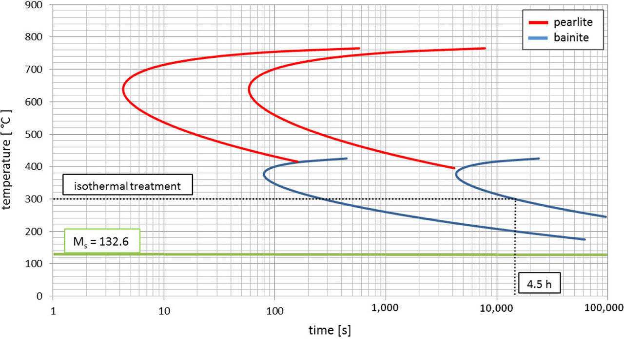
Fig. 1
TTT chart of 9XC steel, with indicated isotherm corresponding to the performed heat treatment. TTT, time–temperature–transformation.
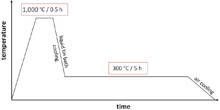
Fig. 2
Heat treatment diagram of the 9XC steel sample analyzed in this research.
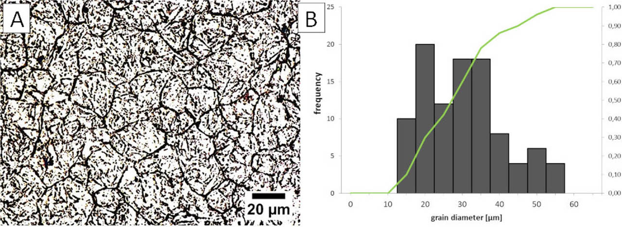
Fig. 3
PAGS analysis using a conventional picric acid solution. (A) Microphotography, light microscopy. (B) Grain diameter distribution. PAGS, prior-austenite grain size.
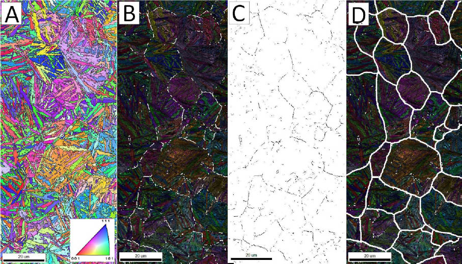
Fig. 4
PAGS analysis using the EBSD technique. (A) Inverse pole figure map. (B) Inverse pole figure and image quality map with the indicated misorientation angles in the range of 20°–40°. (C) Misorientation angles in the range of 20°–40°. (D) Inverse pole figure and image quality map with reconstructed prior-austenite grain boundaries based on misorientation angles and bainitic sheaves orientation. EBSD, electron backscatter diffraction; PAGS, prior austenite grain size.
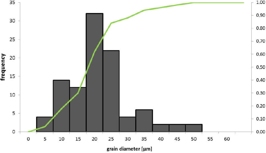
Fig. 5
Grain diameter distribution based on EBSD analysis of PAGS. EBSD, electron backscatter diffraction; PAGS, prior-austenite grain size, green line – cumulative histogram.
Table 2
Comparison of prior-austenite grain size measurements obtained by conventional etching by picric acid solution and by the EBSD technique.
| Method | Measurement counts | x̄, mm | SD, mm | Median, mm | Q1, mm | Q3, mm | ½IQR, mm |
|---|---|---|---|---|---|---|---|
| Conventional etching by picric acid solution | 100 | 27.8 | 10.9 | 26.4 | 18.9 | 34.9 | 8.0 |
| EBSD analysis using misorientation angles (20°–40°) | 100 | 18.7 | 9.2 | 17.8 | 13.9 | 21.8 | 4.0 |
[i] EBSD, electron backscatter diffraction; ½IQR, semi-interquartile range; Q1, first quartile; Q3, third quartile; SD, standard deviation; x̄, average.
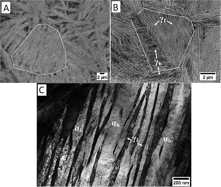
Fig. 6
The microstructure of 9XC steel after isothermal heat treatment. (A) Visible lath morphology of bainite sheaves inside the prior-austenite grain obtained by SEM. (B) Visible austenite with blocky (γb) and film-like (γf) morphologies inside the prior-austenite grain; image obtained by SEM. (C) Bainitic ferrite laths (αb) and film-like austenite (γf) in the area of bainitic sheaves. Images were obtained by TEM (bright field image). SEM, scanning electron microscopy; TEM, transmission electron microscopy.
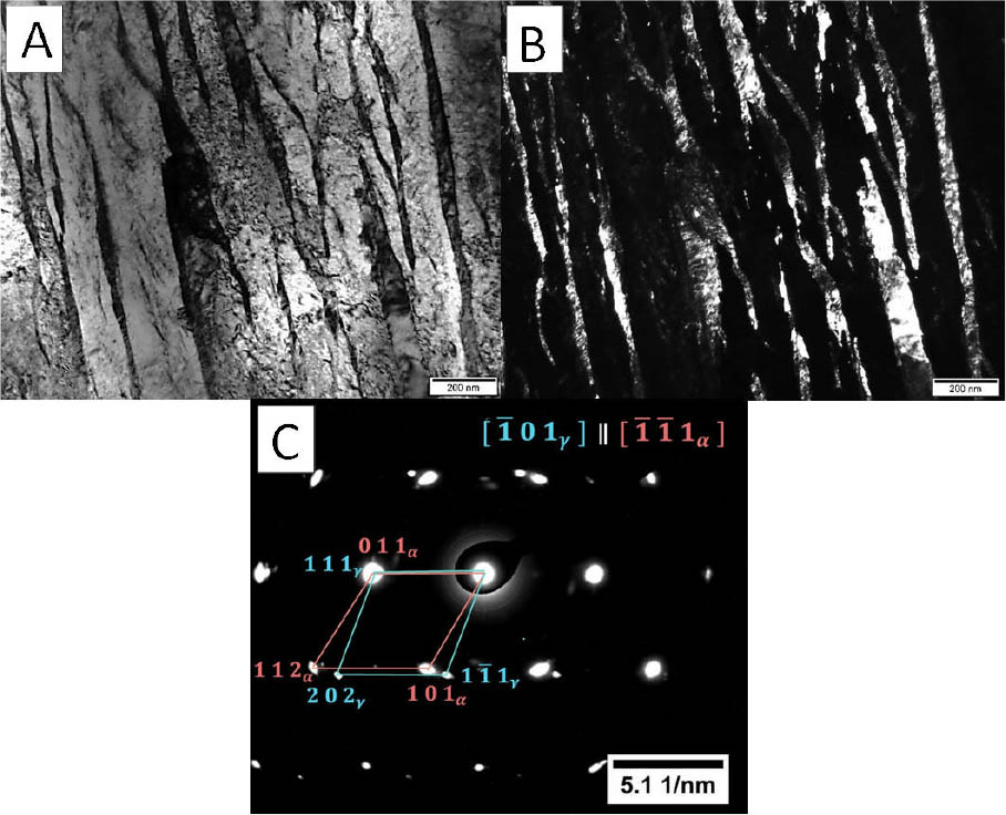
Fig. 7
(A) The bright field image of bainitic sheaves consisting of bainitic ferrite laths and film-like austenite. (B) The dark field image from the austenite reflex ( ). (C) Selected area diffraction pattern with solution from the area presented in panel (A). TEM, 150 kV. TEM, transmission electron microscopy.
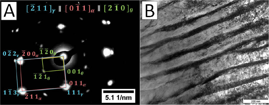
Fig. 8
(A) Selected area diffraction pattern with solution from area presented in panel (B) (B) The bright field image of bainitic sheaves consisting of bainitic ferrite laths, film-like austenite, and cementite precipitations.. TEM, 150 kV. TEM, transmission electron microscopy.
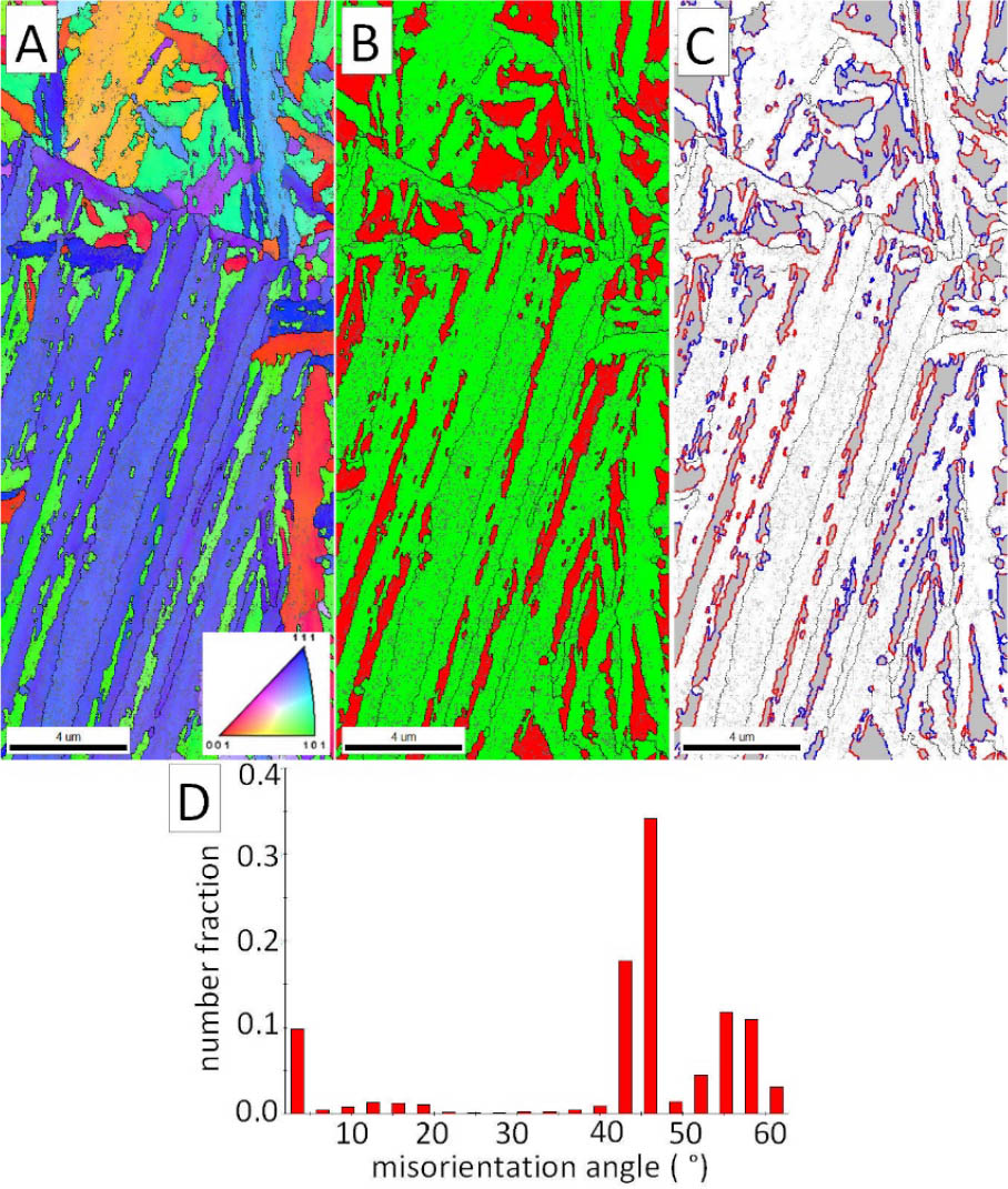
Fig. 9
(A) Inverse pole figure map of 9XC grade steel after isothermal heat treatment. (B) Phase distribution map. Ferrite is marked in green, austenite is marked in red. (C) Phase distribution map (ferrite – white, austenite – gray), with the indicated K–S misorientation angles (43° ± 1) in red and N–W misorientation angles (46° ± 1) in blue. (D) Distribution of the misorientation angles. K–S, Kurdjumov–Sachs; N–W, Nishiyama–Wassermann.
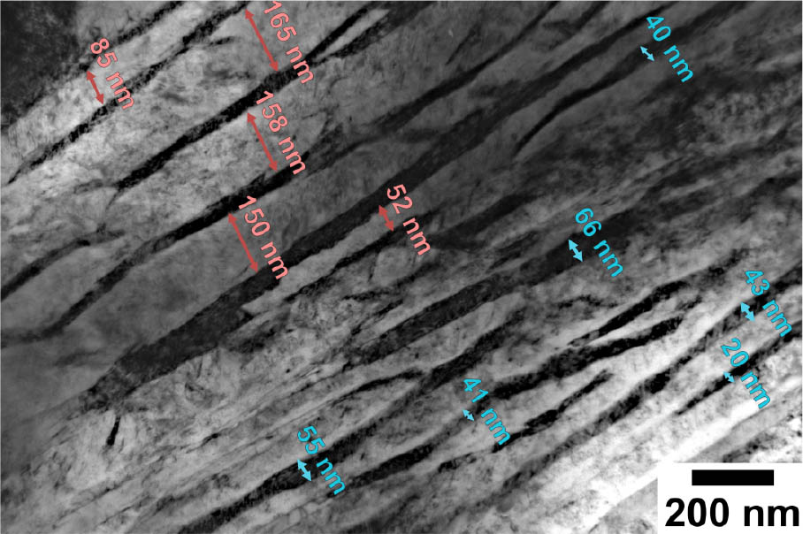
Fig. 10
Example of an image used for phase refinement analysis. TEM, bright field image. TEM, transmission electron microscopy.
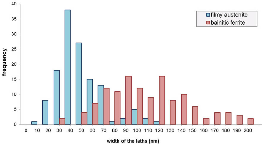
Fig. 11
The width distribution of film-like austenite and bainitic ferrite.
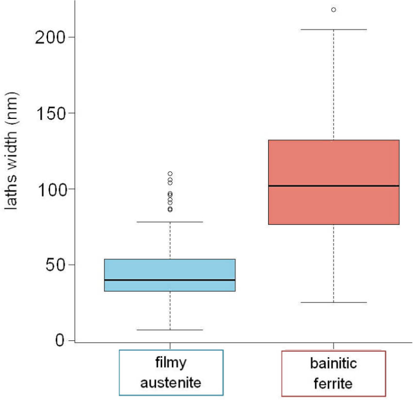
Fig. 12
Box plot of the thicknesses of film-like austenite and bainitic ferrite.
Table 3
Results of measurement of the thicknesses of film-like austenite and bainitic ferrite.
| Phase | Count number | x̄, nm | SD, nm | Median, nm | Q1, nm | Q3, nm | ½IQR, nm |
|---|---|---|---|---|---|---|---|
| Filmy austenite | 131 | 44.6 | 20.3 | 40.0 | 32.5 | 53.4 | 10.4 |
| Bainitic ferrite | 131 | 106.8 | 40.7 | 102.0 | 76.3 | 131.8 | 27.7 |
[i] ½IQR, semi-interquartile range; Q1, first quartile; Q3, third quartile; SD, standard deviation; x̄, xxx.
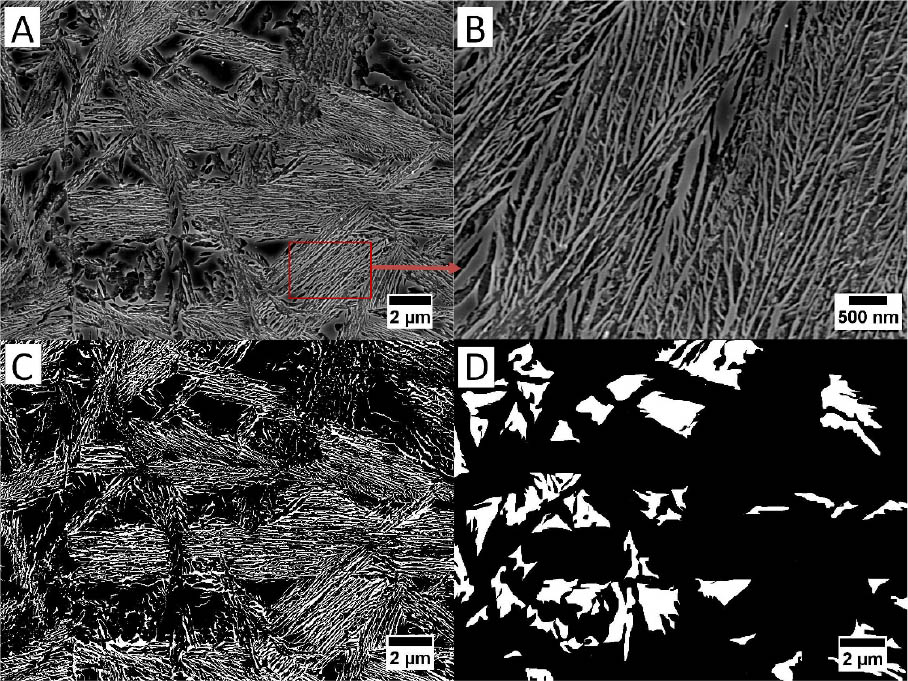
Fig. 13
(A) Example of area intended for qualitative analysis. (B) Magnification of bainitic sheaf. Visible film-like austenite and bainitic ferrite. (C) Graphic image editing intended for film-like austenite measurements. (D) Prepared image for blocky austenite measurements.
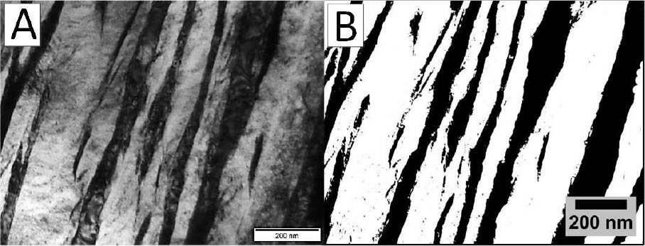
Fig. 14
(A) Bright field image of bainitic sheaf (TEM). (B) Prepared image for area fraction measurement of film-like austenite. TEM, transmission electron microscopy.
Table 4
Measurement results of retained austenite content considering its morphology.
| Method | Measurement areas | Blocky austenite (γb), % | Film-like austenite (γf), % | Total austenite (γb + γf), % | Ratio, γf/γb |
|---|---|---|---|---|---|
| SEM – graphical analysis | 3 | 20.5 ± 3.2 | 23.7 ± 4.1 | 44.2 | 1.16 |
| EBSD – phase distribution map | 3 | 22.3 ± 5.8 | – | – | – |
| TEM – graphical analysis | 5 | – | 24.8 ± 9.1 | – | – |
| TEM + EBSD | – | 22.3 ± 5.8 | 24.8 ± 9.1 | 47.1 | 1.11 |
[i] γb, blocky austenite; γf, film-like austenite; EBSD, electron backscatter diffraction; SEM, scanning electron microscopy; TEM, transmission electron microscopy.