
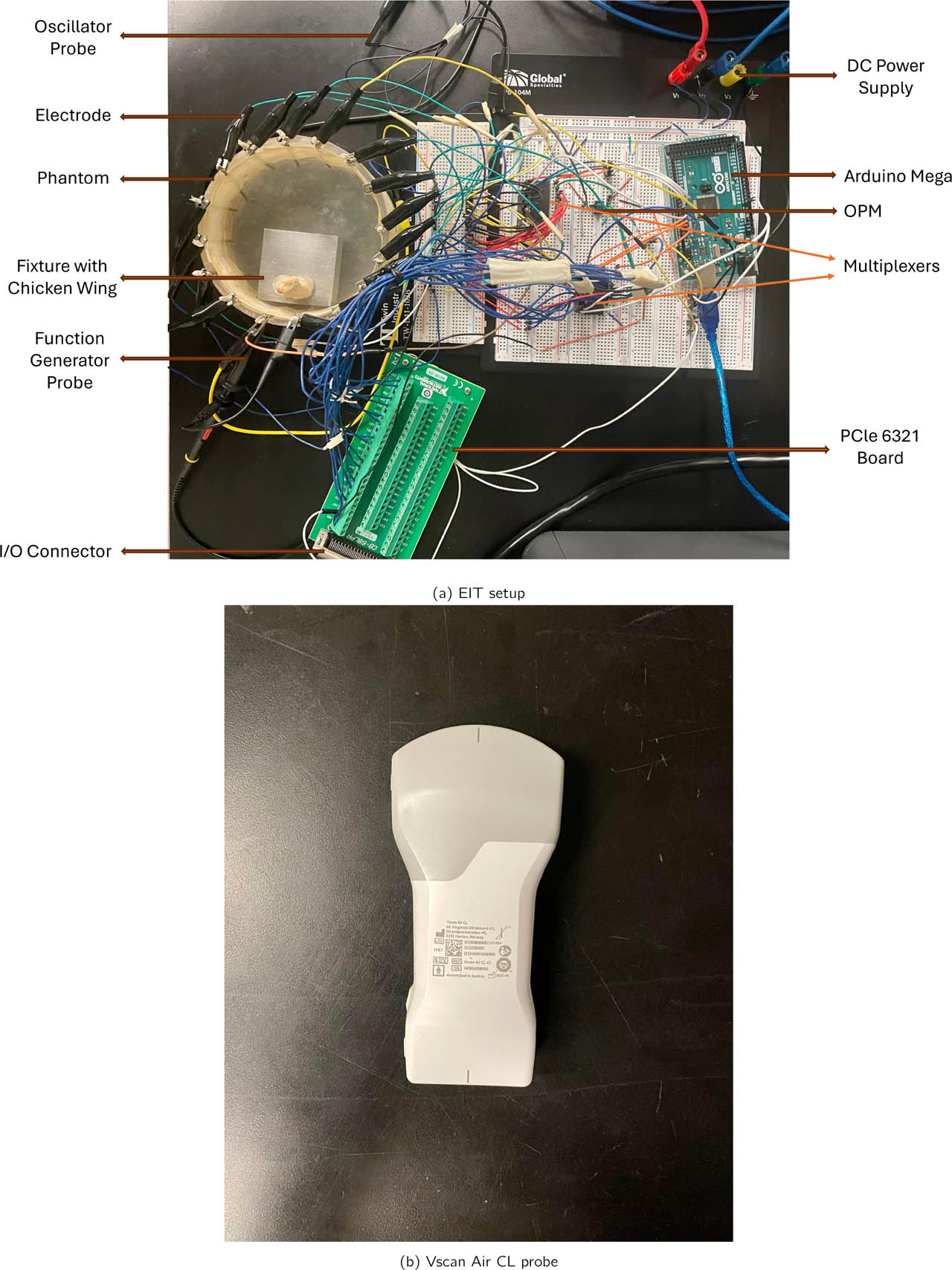
Figure 1:
(a) Experimental phantom setup for EIT–US data acquisition. (b) The ultrasound Vscan Air CL probe is positioned externally above the tissue for co-registered structural imaging. This configuration enables synchronized EIT voltage acquisition and ultrasound-based measurement for multimodal fusion.
Table 1:
Layered Biological Phantom Configuration.
| Layer | Biological Analog | Tissue Composition | Expected US Property | Expected EIT Property |
|---|---|---|---|---|
| L1 | Skin tissue | Epidermis with thin adipose fascia | Hyperechoic skin boundary | Moderate conductivity |
| L2 | Skeletal muscle | Chicken pectoralis major muscle bundle | Hypoechoic, fibrillar texture | Higher conductivity |
| L3 | Connective tissue | Deepdense chicken flexor tendon | Hyperechoic, fibrillar appearance | Lower conductivity |
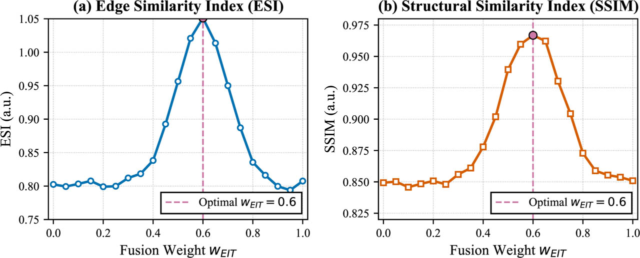
Figure 2:
Sensitivity analysis of fusion weights. (a) Edge Sharpness Index (ESI) as a function of wEIT. (b) Structural Similarity Index (SSIM) as a function of wEIT. The shaded region indicates the stable plateau where both metrics are within 90% of their maximum values. The vertical dashed line marks the selected weight wEIT = 0.6 (wUS = 0.4). Data are shown as mean ± standard deviation across all experimental conditions.

Figure 3:
Overview of the proposed EIT–US fusion pipeline.
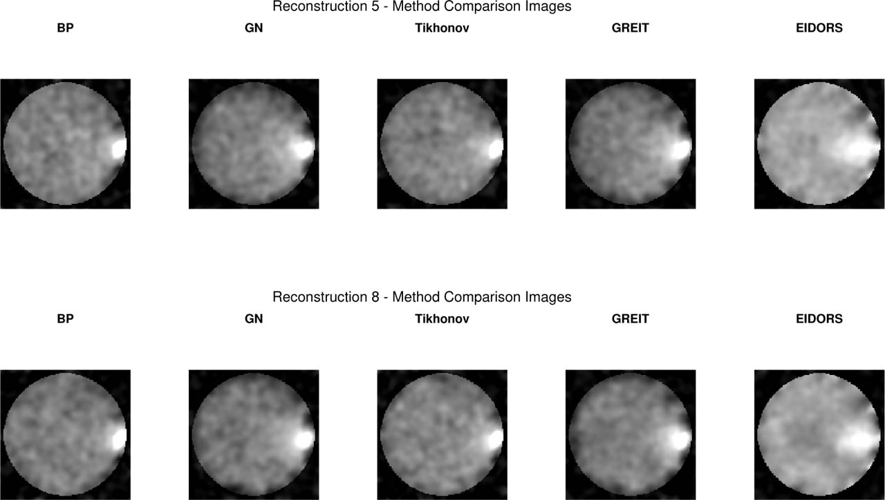
Figure 4:
Comparison of five EIT reconstruction algorithms for two representative excitation settings: (Top) Layer 2 at 10 kHz, 1 V and (Bottom) Layer 2 at 50 kHz, 5 V. (a) Back Projection (BP), (b) Gauss–Newton (GN), (c) Tikhonov (TIK), (d) GREIT, (e) EIDORS-style linear solver. Normalized conductivity Δσ. High-frequency/high-voltage excitation produces higher spatial coherence and improved feature recoverability across all methods.
Table 2:
Comparison of reconstruction quality across algorithms. Values are mean ± SD. FWHM values are reported in pixels (1 pixel = 0.4 mm, corresponding to ≈ 12 mm for GN at ≈ 30 pixels).
| Method | CNR | PSNR (dB) | SSIM | FWHM (pixels) |
|---|---|---|---|---|
| BP | 1.29 ± 0.12 | 10.2 ± 1.1 | 0.918 ± 0.03 | 19.1 ± 3.5 |
| GN | 1.87 ± 0.08 | 12.6 ± 0.9 | 0.950 ± 0.04 | 30.5 ± 2.8 |
| TIK | 1.43 ± 0.10 | 13.4 ± 1.0 | 0.925 ± 0.03 | 22.2 ± 2.4 |
| GREIT | 1.76 ± 0.14 | 11.45 ± 1.3 | 0.937 ± 0.05 | 16.6 ± 2.0 |
| EIDORS-Style | 1.26 ± 0.11 | 9.1 ± 1.0 | 0.891 ± 0.03 | 53.9 ± 2.3 |
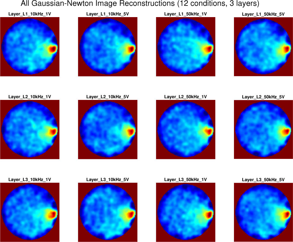
Figure 5:
The EIT system exhibited expected variability across frequency–voltage conditions dominated by the Gauss–Newton algorithm with a cross repeated measurements for sample wing tissue.
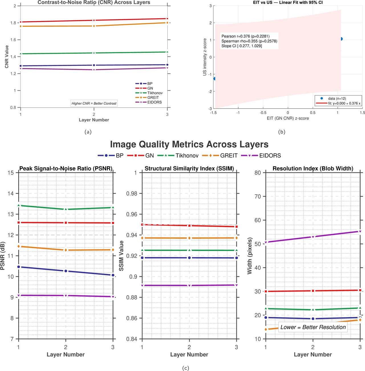
Figure 6:
Layer-dependent reconstruction and cross-modality metrics. (a) CNR across tissue layers for the five reconstruction algorithms. (b) Pearson and Spearman correlation between normalized GN-EIT CNR and ultrasound intensity. (c) PSNR, SSIM, and resolution index across tissue layers for the five reconstruction algorithms.
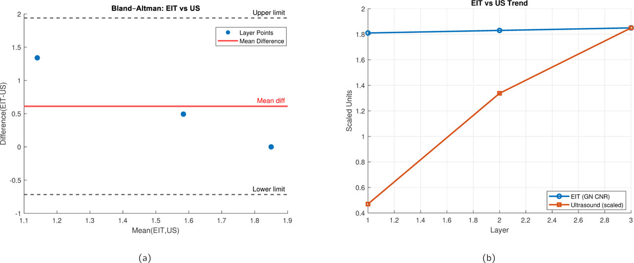
Figure 7:
Statistical agreement between ultrasound and EIT-derived metrics. (a) Bland-Altman plot showing the difference between modalities (EIT - US) against their average. X-axis: Mean of normalized EIT and US values. Y-axis: Difference (EIT - US). Solid line: mean bias (−0.04). Dashed lines: 95% limits of agreement ([−0.36, 0.28]). (b) Comparison of EIT and ultrasound trends across tissue layers. The mean EIT contrast metric (Gauss–Newton CNR) and the corresponding ultrasound-derived intensity index are plotted as a function of layer depth. Ultrasound values are scaled to match the EIT dynamic range to enable direct visual comparison.
Table 3:
Exploratory pairwise comparisons of SSIM across reconstruction methods using two-sided t-tests and Cohen's d effect sizes. Repeated measurements were treated as technical replicates from the same experimental tissue configurations; therefore, the statistical results represent within-experiment comparisons rather than population-level biological inference.
| Comparison | p-value | Effect Size (d) | Significance |
|---|---|---|---|
| GN vs BP | < 0.001 | 2.11 | Strong |
| GN vs TIK | 0.18 | 0.42 | Not significant |
| GN vs GREIT | 0.008 | 1.32 | Significant |
| GN vs EIDORS-Style | 0.09 | 0.55 | Borderline |
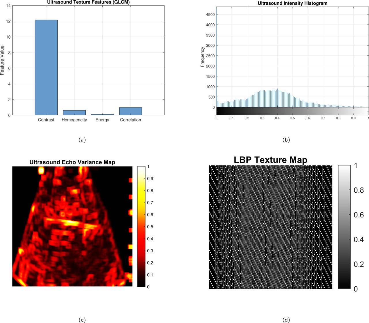
Figure 8:
Representative ultrasound-derived structural and texture analyses of the biological phantom. (a) Ultrasound texture feature map highlighting local speckle and structural heterogeneity, (b) normalized intensity histogram characterizing backscatter distribution within the region of interest, (c) echo variance map emphasizing spatial fluctuations in acoustic scattering, and (d) local binary pattern (LBP) texture map capturing micro-textural variations in tissue structure. Together, these complementary representations provide a multiscale characterization of tissue morphology used to support structural interpretation and fusion with EIT reconstructions.
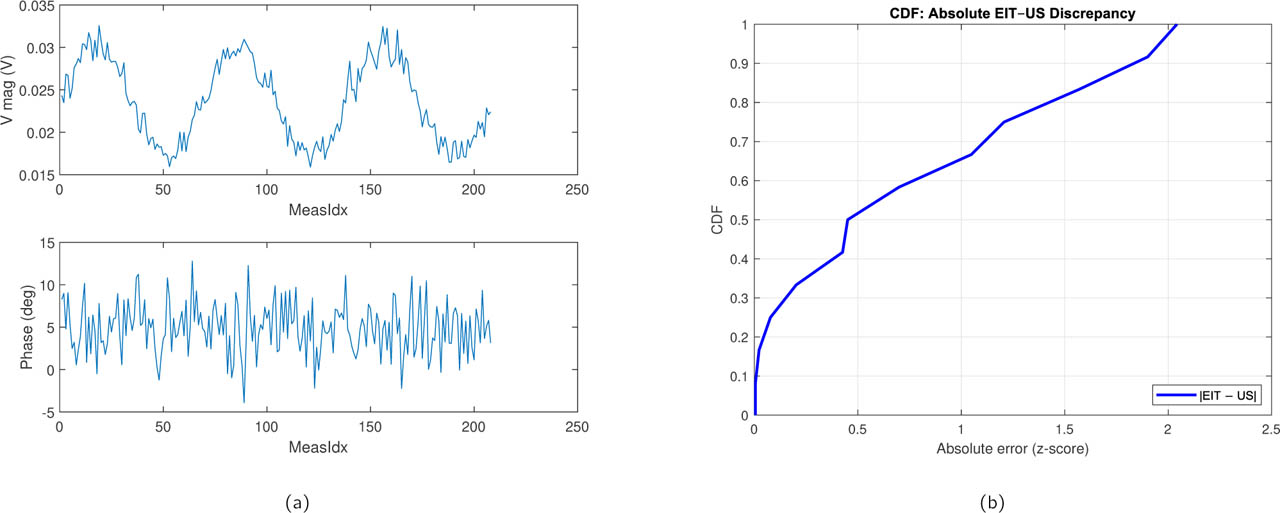
Figure 9:
Modality discrepancy analysis. (a) Representative raw voltage measurements across all drive patterns for a single experimental condition (Layer 2, 50 kHz, 5 V). (b) Cumulative Distribution Functions (CDFs) of the absolute pixel-wise difference between normalized EIT and US images for all three tissue layers. X-axis: Absolute discrepancy (normalized units). Y-axis: Cumulative probability. Layer 1 shows the smallest discrepancy, while Layer 3 exhibits longer tails, confirming deeper tissue challenges.
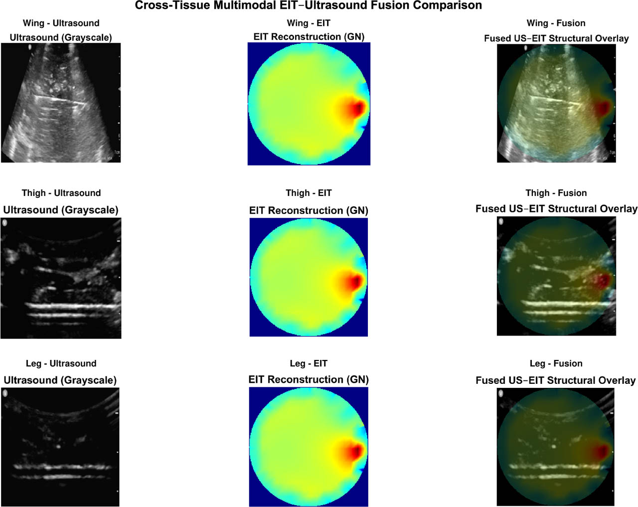
Figure 10:
Cross-anatomical validation of the proposed multimodal EIT–ultrasound fusion framework for a single layer (L1). Representative fused reconstructions are shown for three biological tissue configurations: chicken wing, chicken thigh, and chicken leg. Despite anatomical differences among tissue types, the fused images demonstrate consistent conductivity gradients and clear boundary localization across layers. These observations demonstrate consistency of the processing framework across the three investigated tissue configurations, while larger multi-specimen studies are required to establish biological generalizability.
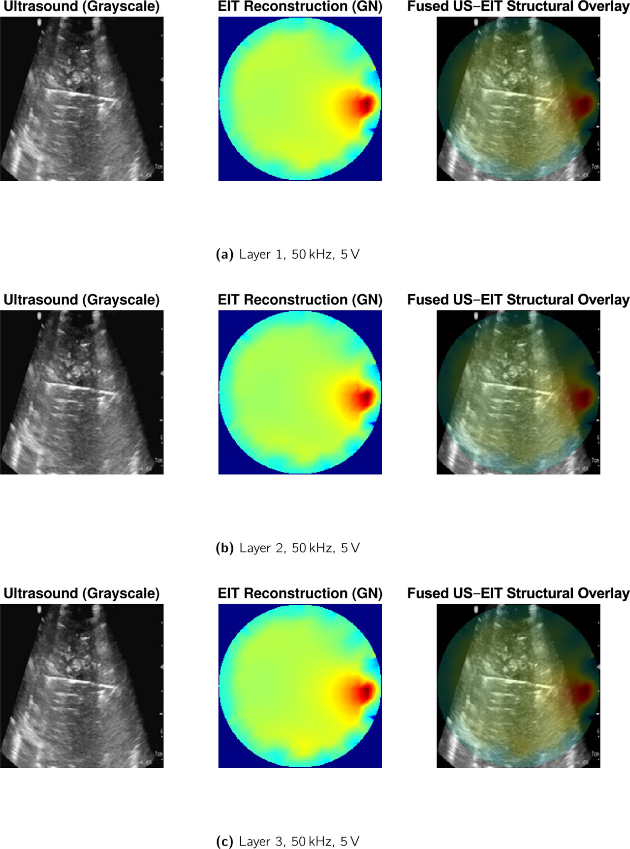
Figure 11:
Fusion results for (a) Layer 1, (b) Layer 2, and (c) Layer 3 at 50 kHz, 5 V excitation for wing tissue layers.
Table 4:
Quantitative evaluation of EIT–US fusion performance across tissue layers. Fusion contrast is defined as the normalized gradient magnitude at the layer interface. Values are mean ± SD across all excitation conditions (n = 12).
| Layer | EIT CNR | US Intensity | Fusion Contrast | Fusion SSIM |
|---|---|---|---|---|
| L1 | 1.85 ± 0.04 | 0.42 ± 0.03 | 0.61 ± 0.05 | 0.78 ± 0.02 |
| L2 | 1.83 ± 0.03 | 0.36 ± 0.04 | 0.55 ± 0.04 | 0.75 ± 0.03 |
| L3 | 1.81 ± 0.05 | 0.29 ± 0.05 | 0.47 ± 0.06 | 0.71 ± 0.04 |
Table 5:
Cross-anatomical consistency of multimodal fusion performance across chicken tissue configurations. Values are mean ± SD.
| Tissue Type | EIT CNR | Fusion CNR | Fusion SSIM | ESI |
|---|---|---|---|---|
| Chicken Wing | 1.72 ± 0.09 | 2.18 ± 0.11 | 0.94 ± 0.02 | 0.66 ± 0.05 |
| Chicken Thigh | 1.69 ± 0.08 | 2.14 ± 0.10 | 0.93 ± 0.02 | 0.64 ± 0.04 |
| Chicken Leg | 1.65 ± 0.10 | 2.09 ± 0.12 | 0.92 ± 0.03 | 0.63 ± 0.05 |
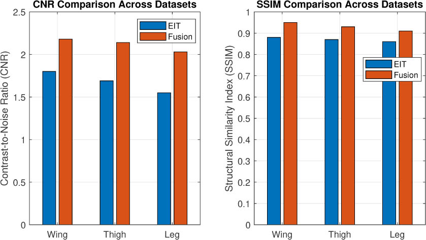
Figure 12:
Summary comparison of reconstruction performance across chicken wing, thigh, and leg tissue datasets. Average contrast-to-noise ratio (CNR) and structural similarity (SSIM) are shown for EIT-only reconstruction and the proposed multimodal fusion framework. The fusion framework shows consistent performance trends across the three investigated anatomical configurations, providing preliminary evidence of cross-anatomical consistency within the experimental dataset. Larger multi-specimen studies are required to establish biological generalizability.
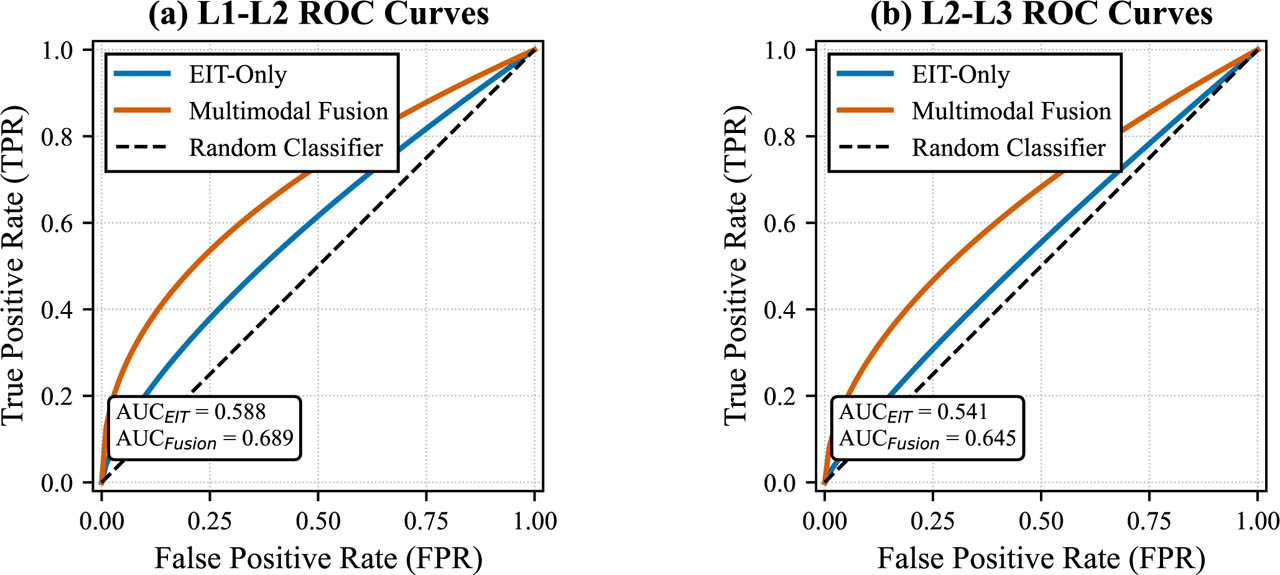
Figure 13:
Receiver operating characteristic (ROC) curves for layer boundary detection. (a) L1–L2 (superficial fascia–muscle) interface. (b) L2–L3 (muscle–tendon) interface. Blue curves: EIT-only GN reconstruction. Red curves: fused images. The diagonal dashed line represents chance performance (AUC = 0.5). Fusion consistently improves AUC, sensitivity, and specificity across both interfaces.