
Figure 1:
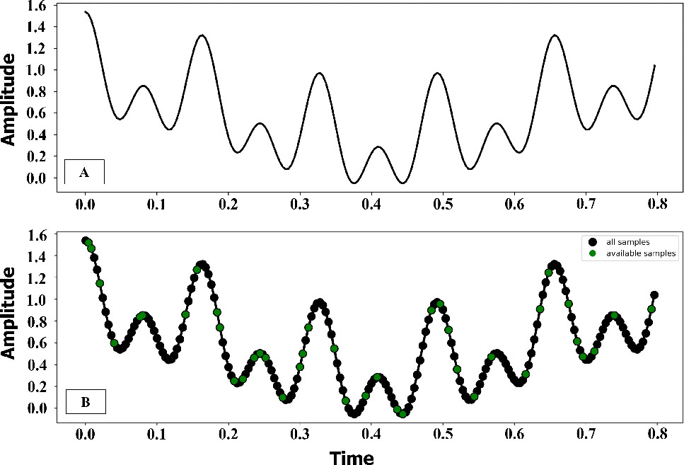
Simulate the wave signals from three frequencies of 10, 50, and 100 kHz with (A) the sum of the signal and (B) the discrete point in the signal with a threshold of 0.2.
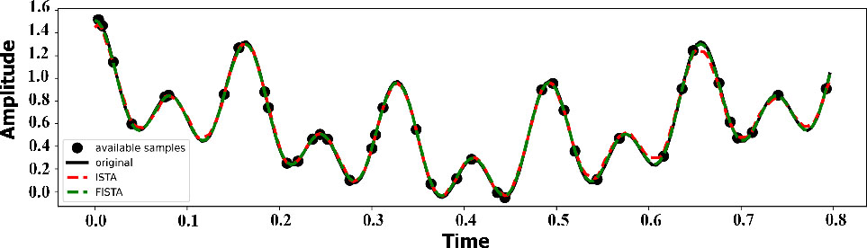
Figure 2:
Reconstructed signal from ISTA and FISTA iterative method.
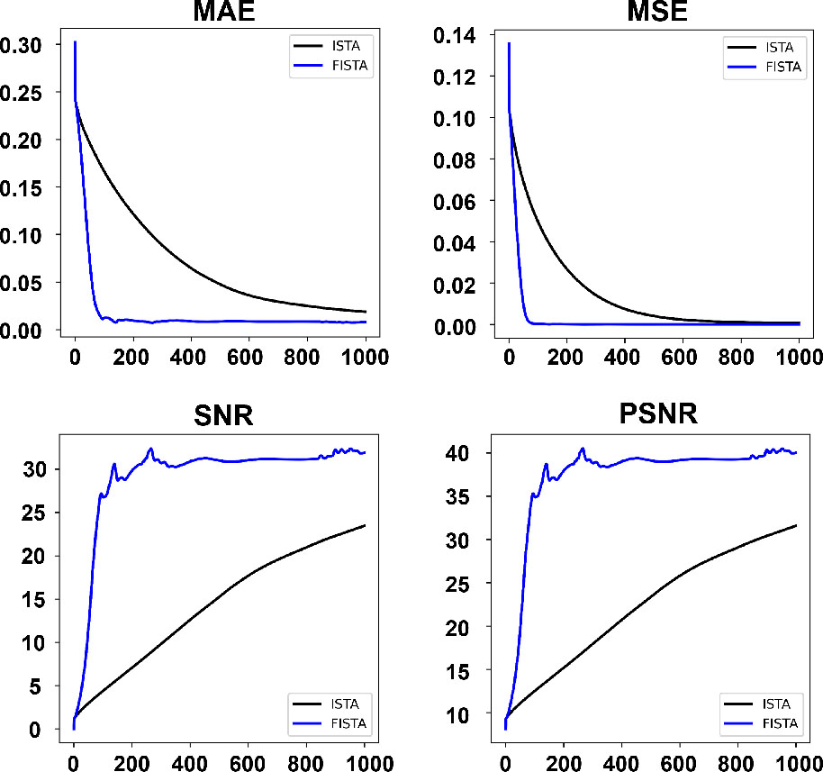
Figure 3:
Evaluation of ISTA and FISTA performance based on MAE, MSE, SNR, and PSNR metrics over iterations.
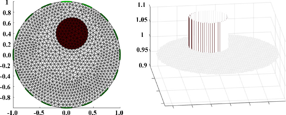
Figure 4:
16-electrode model simulates an abnormal object with a radius of 0.3 in the phantom mesh (left) and intensity conductivity (right).
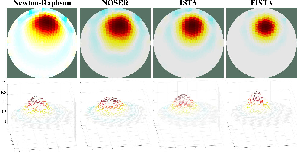
Figure 5:
Reconstructed EIT image (top) and conductivity intensity (bottom) using Newton-Raphson, NOSER, ISTA, and FISTA regularization methods, respectively
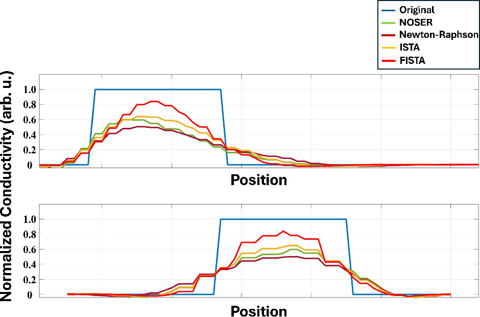
Figure 6:
Normalized conductivity profile through the center of the object vertically (top) and horizontally (bottom).
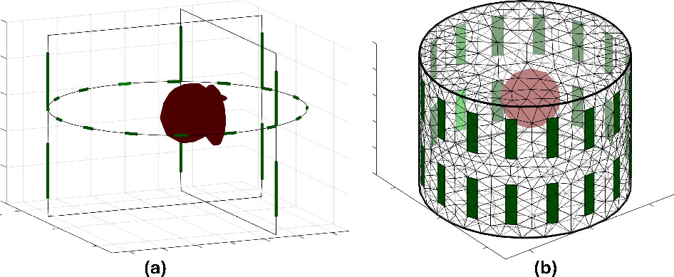
Figure 7:
3D simulation model 32 electrodes (2 rings) of an irregular spherical object with radius 0.3 in phantom with (a) in three axes and (b) in three-dimensional space.
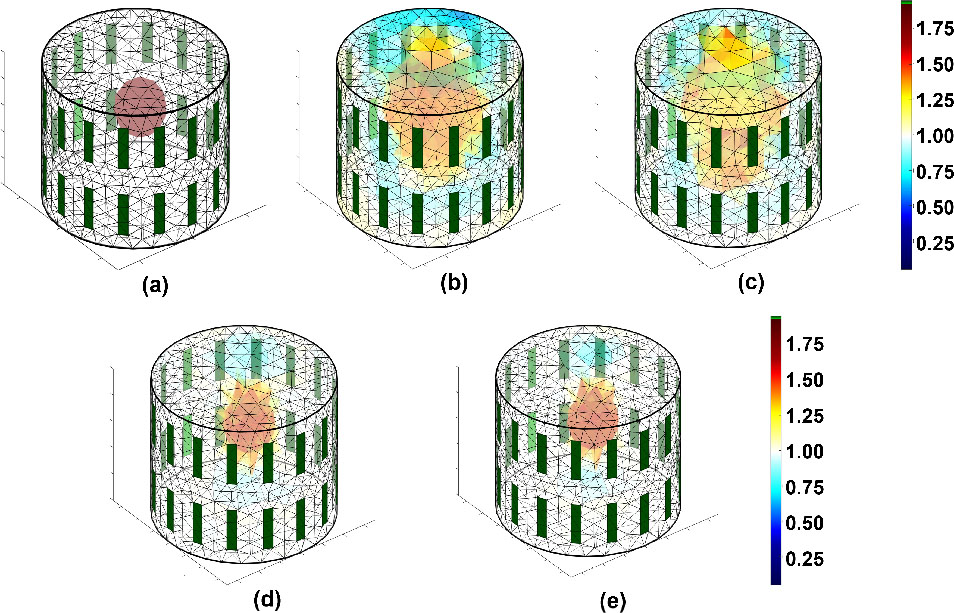
Figure 8:
3D EIT reconstruction using iterative methods with (a) original object, (b) Newton-Raphson, (c) NOSER, (d) ISTA, and (e) FISTA with corresponding conductivity scale.
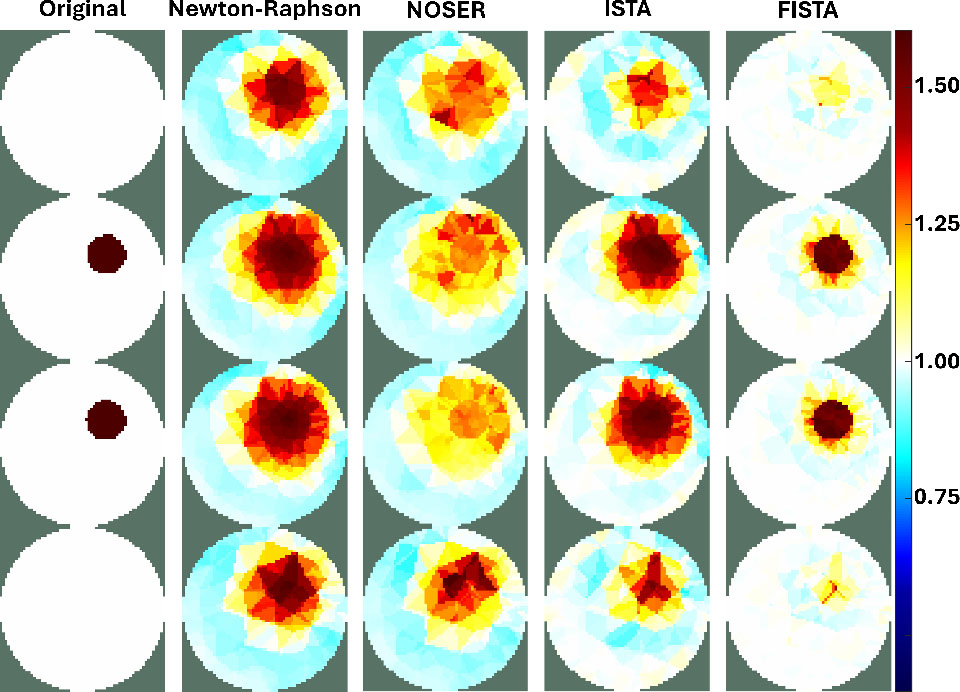
Figure 9:
Cross-section of the 3D EIT image shown in Fig. 8 corresponds to the iterative methods from left-to-right original object, Newton-Raphson, NOSER, ISTA, and FISTA, respectively.
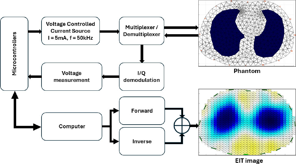
Figure 10:
Process of signal acquisition and image reconstruction of the EIT device.
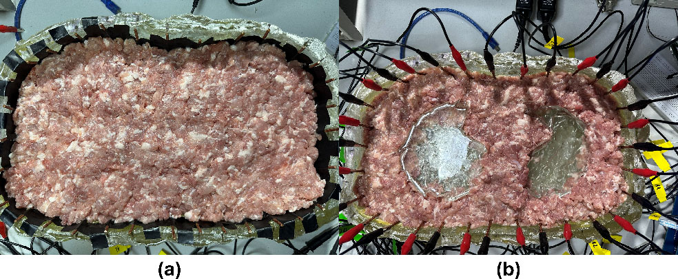
Figure 11:
Phantom model with ground pork meat and acrylic resin objects simulating the lung shape with (a) without objects and (b) with objects.
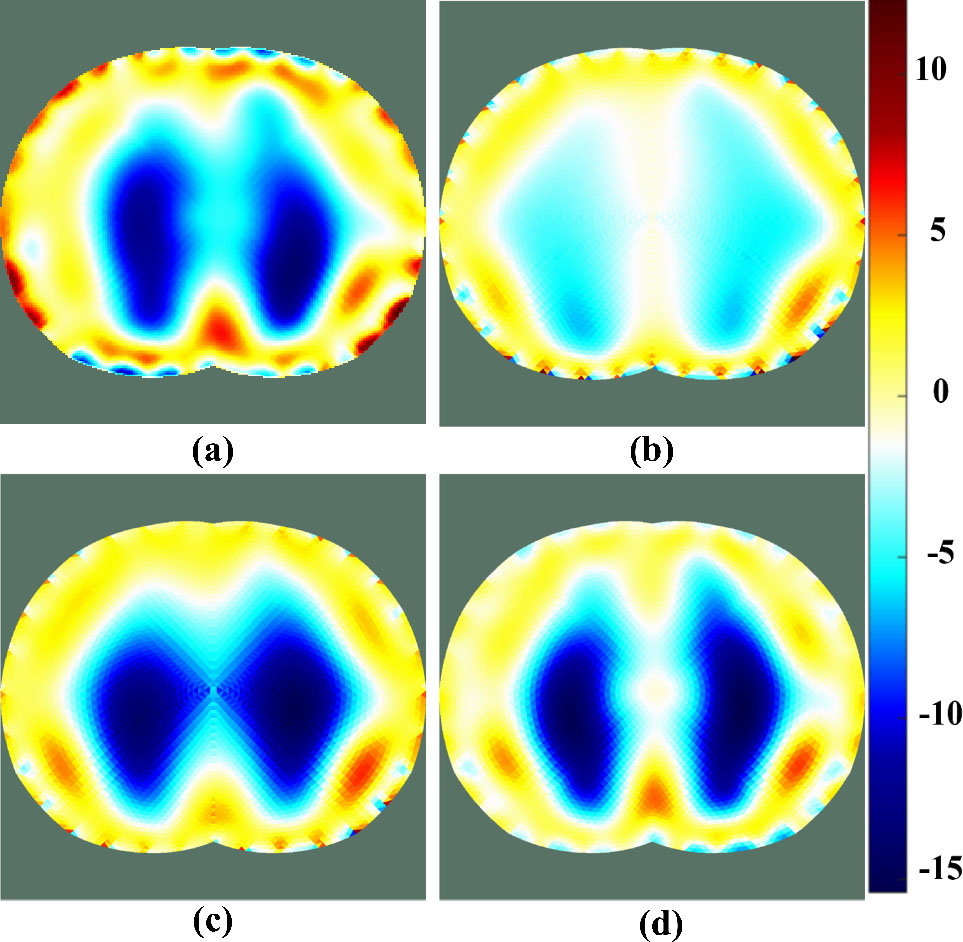
Figure 12:
EIT image reconstructed from the lung simulation phantom using iterative methods with (a) Newton-Raphson, (b) NOSER, (c) ISTA, and (d) FISTA.
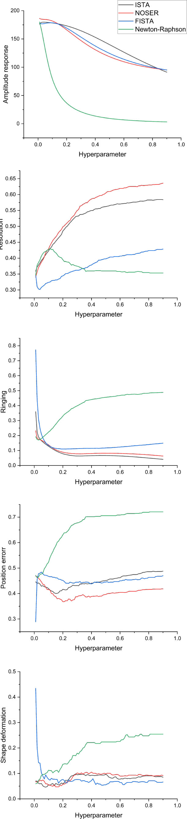
Figure 13:
EIT image evaluation parameters reconstructed when tuning hyperparameters.