
Table 1
Descriptive statistics using IMSS data (September 2018)
| Variables | All | Border region | Non-border region |
|---|---|---|---|
| No. of municipalities | 413 | 18 | 395 |
| Employment: All | 19,035,280 | 2,050,744 | 16,984,536 |
| % Employment: Men | 62.09 | 59.85 | 62.37 |
| % Employment: Women | 37.91 | 40.15 | 37.63 |
| % Employment: Firm size 1–5 | 6.77 | 5.31 | 6.95 |
| % Employment: Firm size 6–50 | 20.89 | 15.96 | 21.48 |
| % Employment: Firm size 51+ | 72.34 | 78.73 | 71.57 |
| % Employment: Age < 30 | 33.37 | 35.83 | 33.07 |
| % Employment: Age 30–59 | 63.75 | 61.91 | 63.97 |
| % Employment: Age 60+ | 2.88 | 2.26 | 2.95 |
| % Earning < MXN 180 daily | 39.83 | 30.64 | 40.94 |
| Avg. daily income < MXN 180 daily | USD 121.6 | USD 129.4 | USD 120.9 |
| Avg. monthly income: All | 9,427 | 10,131 | 9,365 |
| Avg. monthly income: Men | 9,949 | 11,006 | 9,856 |
| Avg. monthly income: Women | 8,470 | 8,819 | 8,440 |
| Avg. monthly income: Firm size 1–5 | 4,897 | 5,281 | 4,863 |
| Avg. monthly income: Firm size 6–50 | 6,992 | 7,769 | 6,924 |
| Avg. monthly income: Firm size 51+ | 10,890 | 11,018 | 10,878 |
| Avg. monthly income: Age < 30 | 7,116 | 7,716 | 7,063 |
| Avg. monthly income: Age 30–59 | 10,626 | 11,547 | 10,545 |
| Avg. monthly income: Age 60+ | 9,192 | 9,196 | 9,191 |
| Avg. population | 1,351,532 | 927,028 | 1,388,767 |
| % People in poverty | 38.1 | 30.8 | 38.8 |
| # Social needs (poverty measure) | 2.0 | 1.8 | 2.0 |
| % People in extreme poverty | 5.2 | 2.3 | 5.5 |
| % People in income poverty | 8.8 | 10.0 | 8.7 |
| % People behind in school | 15.0 | 14.3 | 15.1 |
| % People attending school (15–24 years old) | 46.9 | 44.6 | 47.1 |
| % People (25+ years old) with at least college degree | 15.7 | 12.5 | 16.0 |
| % Households receiving remittances | 9.5 | 10.4 | 9.4 |
| % Women who work (20–65 years old) | 44.6 | 49.0 | 44.2 |
| % Men who work (20–65) | 82.5 | 83.6 | 82.4 |
| % Employment in manufacturing (20–65) | 16.4 | 31.2 | 15.1 |
| % Informal employment (20–65) | 45.5 | 32.2 | 46.7 |
[i] Notes: Authors’ calculations. Statistics related to employment and earnings are from IMSS data, and statistics on poverty, school attendance, remittances, share in manufacturing, and informality are from the Encuesta Intercensal (2015) and Coneval (2019).
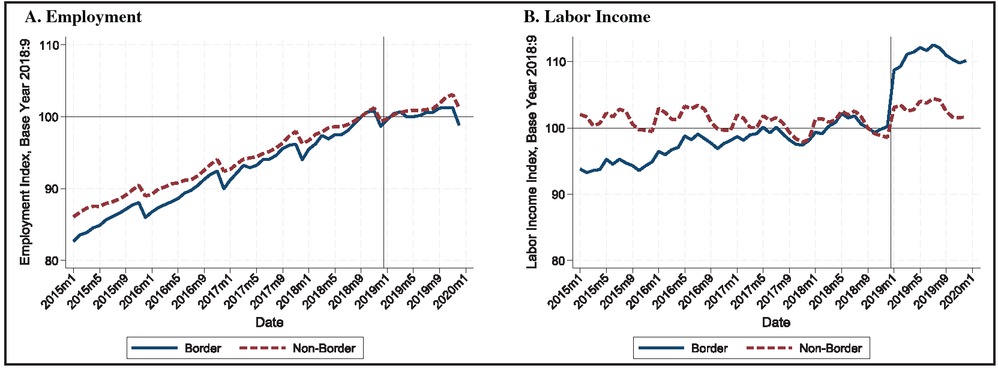
Figure 1
Employment and labor income between border and non-border regions.
Notes: Authors’ calculations using IMSS data restricted to municipalities with at least 50,000 inhabitants. Border refers to the 18 municipalities in the treatment group. Labor income is deflated using the same Consumer Price Index for both regions.
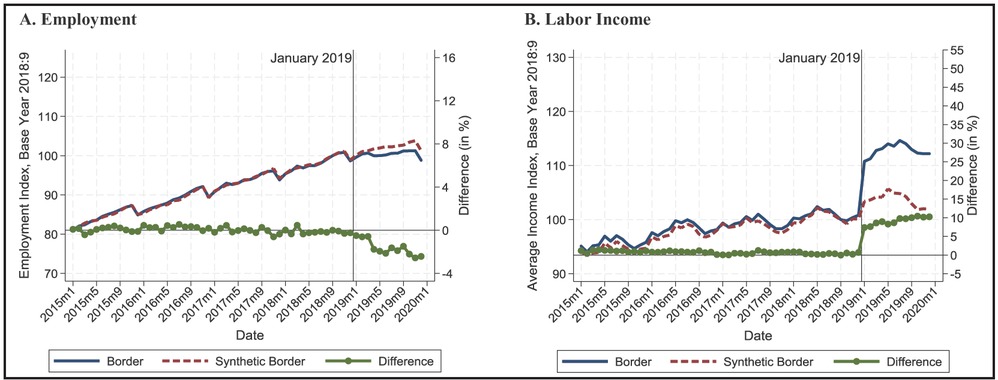
Figure 2
Synthetic control method (SCM) results, 2015–2019.
Notes: Authors’ calculations. The SCM is applied to each of the 18 municipalities in the treated group. The trends for the treatment and synthetic group are then obtained using the 2015 population as weights. The base period is September 2018; the policy was implemented in January 2019.
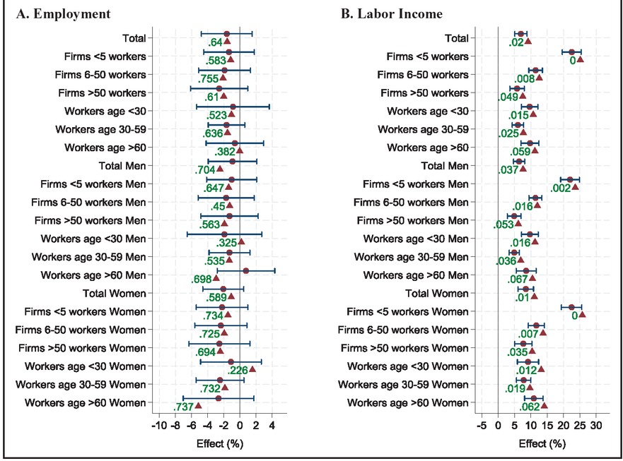
Figure 3
Heterogeneity results, 2015–2019.
Notes: Authors’ calculations. The synthetic control method (SCM) is implemented for each outcome variable on the y-axis for the 18 municipalities in the treated group. The 95% confidence intervals (robust and clustered at the municipality level) are obtained from a regression with fixed effects for time and treatment group (18) using the weights obtained in the SCM. The p-values from the placebo tests are shown next to the triangles. Placebos with a RMSPE larger than 2.5 times the treated unit are omitted.
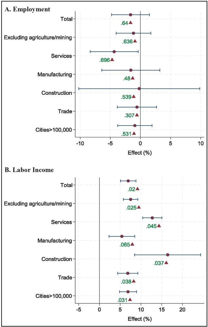
Figure 4
Heterogeneity results by economic sector, 2015–2019.
Notes: Authors’ calculations. The synthetic control method (SCM) is implemented for each outcome variable on the y-axis for the 18 municipalities in the treated group. The 95% confidence intervals (robust and clustered at the municipality level) are obtained from a regression with fixed effects for time and treatment group (18), using the weights obtained in the SCM. The p-values from the placebo tests are shown besides the triangles. Placebos with a RMSPE larger than 2.5 times the treated unit are omitted.
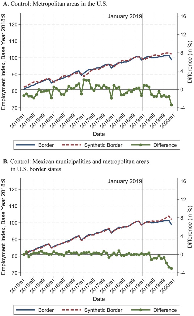
Figure 5
Robustness test using metropolitan areas in the United States as controls, 2015–2019.
Notes: Authors’ calculations. The synthetic control method is implemented for each outcome variable on the x-axis for the 18 municipalities in the treated group. Control group in panel A constructed from metropolitan areas in the US control group in panel B constructed from municipalities in Mexico and all metropolitan areas in US border states. The difference is not statistically significant.
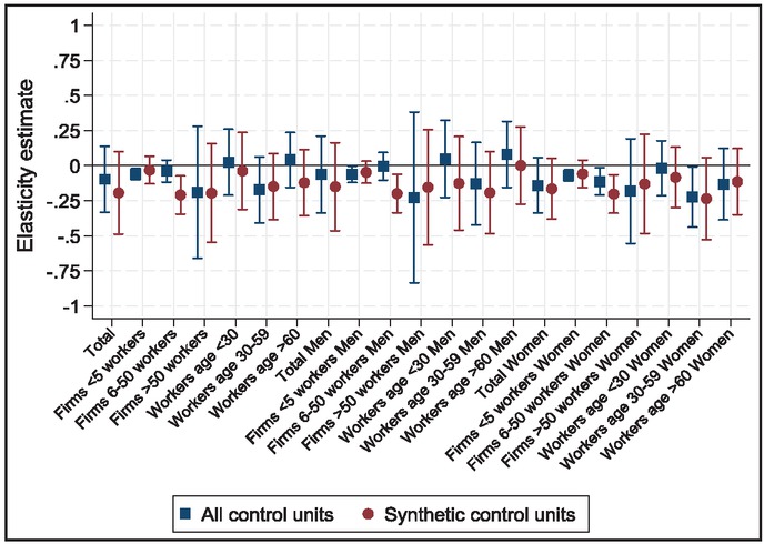
Figure 6
Instrumental variable results, 2015–2019.
Notes: Authors’ calculations. 95% confidence intervals. “All control units” is a regression for all units in the treatment and control groups; the dependent variable is the employment index and the independent variable is the labor income index in 2019, instrumented with a dummy variable for the municipalities in the border region. The regression includes fixed effects of time and municipality as well as the control variables summarized in Table 1 interacted with a trend and state trends, and the fraction of workers in the municipality with daily earnings less than MXN 180 interacted with a trend. Regression is weighted by the population in 2015. The results for “synthetic control units” uses only fixed effects for time and the 18 treatment groups, but weighted by the synthetic control weights interacted with population in 2015.
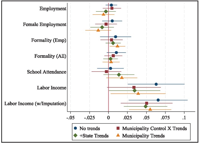
Figure 7
Labor force survey results using repeated cross-sections, 2015–2019.
Notes: Authors’ calculations using ENOE data. Each dot is the coefficient for the border region in 2019 for different regressions; the outcome variables are shown on the y-axis. The regression is at the individual level. Control variables include fixed effects by time and municipality, individual age, gender, schooling, and marital status. Municipality Control X Trends: Trends are interacted with controls at the municipality level. Municipality Trends: municipality fixed effects are interacted with a trend.