
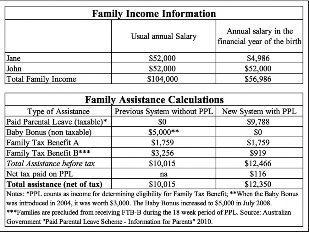
Figure 1
Family assistance example.
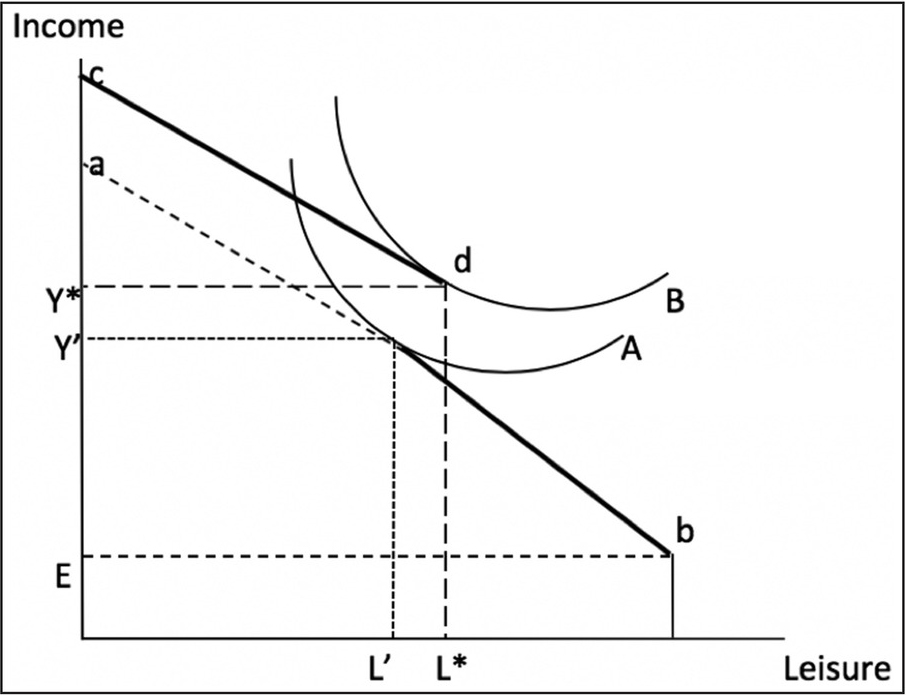
Figure 2
Predicted effect of maternal labor supply pre birth.
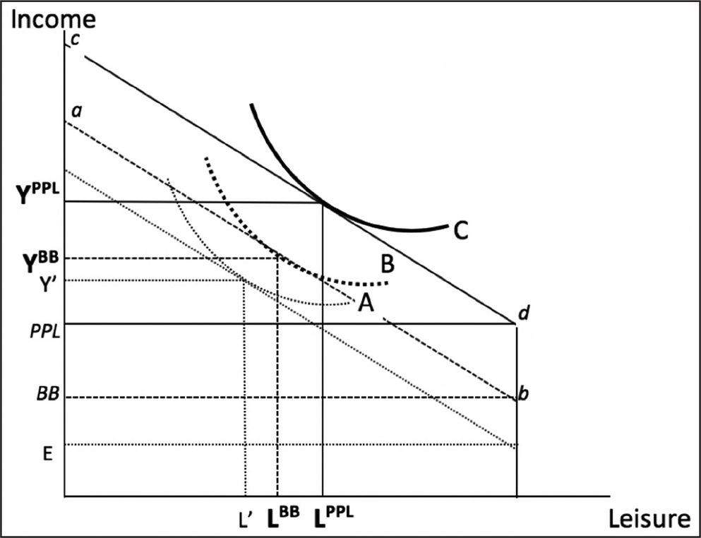
Figure 3
Predicted effect of maternal labor supply post birth.
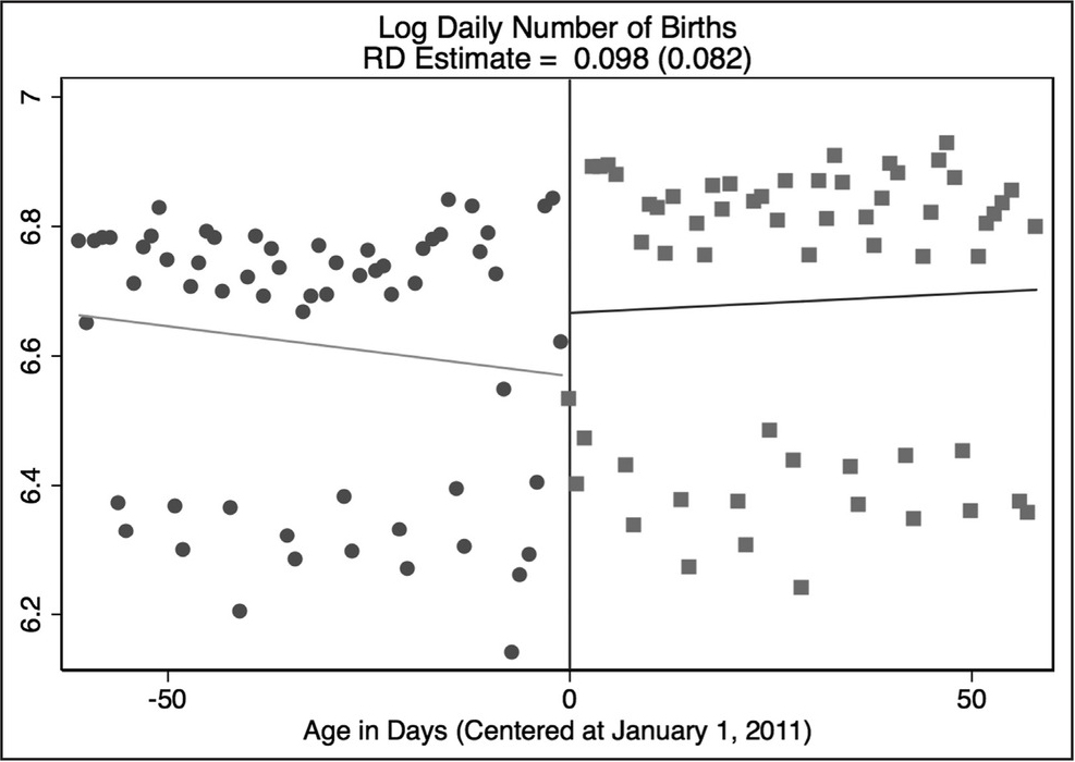
Figure 4
Births discontinuity. Notes: The log of the number of children born to mothers from November 1 2010 to February 28 2011, and separate linear fits on each side of the January 1 2011 cutoff. The vertical line denotes the PPL cutoff of January 1 2011, normalized to 0.
Table 1
Discontinuity in births at the January 1 2011, threshold
| 2–2 m | 2–2 m | 2–2 m | 1–1 m | 1–1 m | 1–1 m | |
|---|---|---|---|---|---|---|
| Births | 0.098 | 0.055 | 0.120 | 0.127 | 0.043 | -0.047 |
| (0.082) | (0.125) | (0.166) | (0.120) | (0.168) | (0.189) | |
| N (number of days) | 120 | 120 | 120 | 62 | 62 | 62 |
| Linear term in m | Yes | Yes | Yes | Yes | Yes | Yes |
| Quadratic term in m | No | Yes | Yes | No | Yes | Yes |
| Cubic term in m | No | No | Yes | No | No | Yes |
[i] Notes: Each coefficient reported is the estimated discontinuity in the daily number of logged births at the threshold as a result of the PPL scheme. The “m” in each column heading stands for months, and represents the number of months on each side of the threshold. Each coefficient is from a different regression. Robust standard errors are in parentheses.
***p < 0.01, **p < 0.05, *p < 0.1.
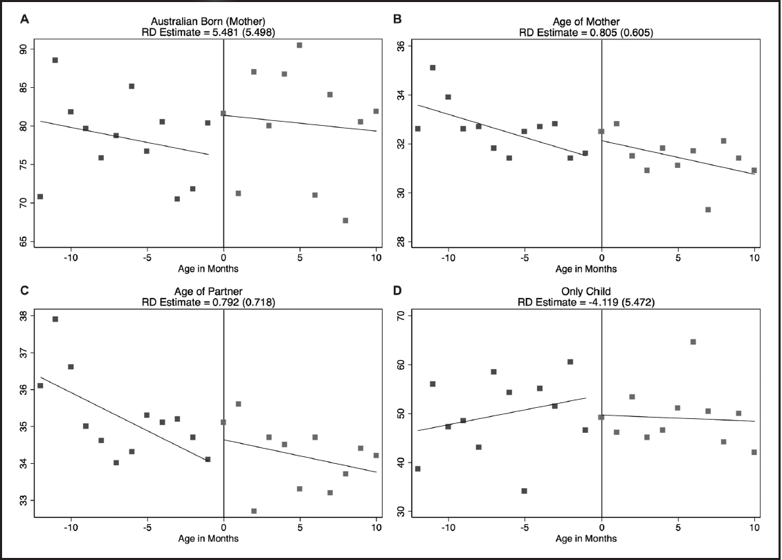
Figure 5
Balance in covariates around the January 1 2011 threshold: (A) Percentage of mothers who are Australian born. (B) Average age of the mother. (C) Average age of the mother’s partner. (D) Percentage of mothers with only one child.
Table 2
Descriptive statistics of analysis variables
| Pre-PPL | Post-PPL | |
|---|---|---|
| Panel I: outcomes | ||
| Percentage receiving Baby Bonus | 68.13 (5.647) | 19.00 (8.183) |
| Average number of weeks stopped work before birth | 3.858 (0.979) | 3.864 (0.775) |
| Average number of hours worked before stopped for birth | 30.07 (2.021) | 31.07 (2.306) |
| (per week) | ||
| Average age of the child when the mother returned to | 30.41 (5.804) | 12.54 (7.712) |
| work (in weeks) | ||
| Average number of hours worked in all jobs (per week) | 16.04 (3.865) | 4.564 (3.507) |
| N (number of months) | 11 | 12 |
| Panel II: covariates | ||
| Australian born (mother) | 78.33 (5.584) | 80.18 (7.324) |
| Age of partner | 35.24 (1.154) | 34.22 (0.877) |
| Age of mother | 32.59 (1.067) | 31.45 (0.943) |
| Only child | 49.48 (8.067) | 49.33 (6.090) |
| N (number of months) | 11 | 12 |
[i] Notes: Data on each outcome was provided by the Australian Bureau of Statistics. The covariates in Panel II are: the percentage of mothers who are Australian born, the average age of the mother’s partner, the average age of the mother and the percentage of mothers with only one child. Means and standard deviations (in parentheses) are presented.
Table 3
Baby Bonus receipt
| 12–12 m | 12–12 m | 12–12 m | |
|---|---|---|---|
| Baby bonus | -46.24*** (6.595) | -44.52*** (10.11) | -43.06*** (7.703) |
| N (number of months) | 23 | 23 | 23 |
| Controls | Yes | Yes | Yes |
| Linear term in m | Yes | No | No |
| Quadratic term in m | No | Yes | No |
| Cubic term in m | No | No | Yes |
[i] Notes: The coefficient reported is the estimated discontinuity in Baby Bonus Receipt as a result of the PPL scheme. The “m” in the column heading stands for months. An observation is the outcome rate for a 1-month age cell. Controls include the percentage of mothers in each age cell that are Australian born, the average age of the mother in each age cell, the average age of the partner in each age cell, and the percentage of mothers with one child in each age cell. Estimates are weighted by the population, and robust standard errors are in parentheses.
***p < 0.01, **p < 0.05, *p < 0.1.
Table 4
The effect of PPL on maternal labor market outcomes
| Hours before birth (1) | Weeks stop before birth (2) | Age of child return (3) | Hours worked, November 2011 (4) | |
|---|---|---|---|---|
| Panel I | ||||
| PPL | 0.046 (0.059) | -0.171 (0.195) | 0.905** (0.357) | -0.202 (0.221) |
| N (number of months) | 23 | 23 | 23 | 23 |
| Controls | Yes | Yes | Yes | Yes |
| Linear term in m | Yes | Yes | Yes | Yes |
| Panel II | ||||
| PPL | 0.042 (0.112) | -0.324 (0.272) | 0.036 (0.207) | -0.101 (0.390) |
| N (number of months) | 23 | 23 | 23 | 23 |
| Controls | Yes | Yes | Yes | Yes |
| Quadratic term in m | Yes | Yes | Yes | Yes |
[i] Notes: The coefficient reported is the estimated discontinuity in the outcome as a result of the PPL scheme. Each coefficient is from a different regression. An observation is the outcome rate for a 1-month age cell. Controls include the percentage of mothers in each age cell that are Australian born, the average age of the mother in each age cell, the average age of the partner in each age cell, and the percentage of mothers with one child in each age cell. Estimates are weighted by the population, and robust standard errors are in parentheses.
***p < 0.01, **p < 0.05, *p < 0.1.
Table 5
Average age of the child when the mother returned to work, by income quintile
| First quintile | Second quintile | Third quintile | Fourth quintile | Fifth quintile | |
|---|---|---|---|---|---|
| Panel I | |||||
| Average age of child | -0.153 | 1.012 | 1.248 | 0.171 | 0.529 |
| (0.771) | (0.675) | (1.074) | (0.529) | (0.466) | |
| N (number of months) | 23 | 23 | 23 | 23 | 23 |
| Controls | Yes | Yes | Yes | Yes | Yes |
| Linear term in m | Yes | Yes | Yes | Yes | Yes |
| Panel II | |||||
| Average age of child | 0.067 | 0.325 | 1.160 | 0.965 | 0.219 |
| (1.325) | (0.697) | (1.480) | (0.764) | (0.837) | |
| N (number of months) | 23 | 23 | 23 | 23 | 23 |
| Controls | Yes | Yes | Yes | Yes | Yes |
| Quadratic term in m | Yes | Yes | Yes | Yes | Yes |
[i] Notes: Each coefficient reported is the estimated discontinuity in the outcome as a result of the PPL scheme. Each coefficient is from a different regression. An observation is the outcome rate for a 1-month age cell. Controls include the percentage of mothers in each age cell that are Australian born, the average age of the mother in each age cell, the average age of the partner in each age cell, and the percentage of mothers with one child in each age cell. Estimates are weighted by the population, and robust standard errors are in parentheses.
***p < 0.01, **p < 0.05, *p < 0.1.
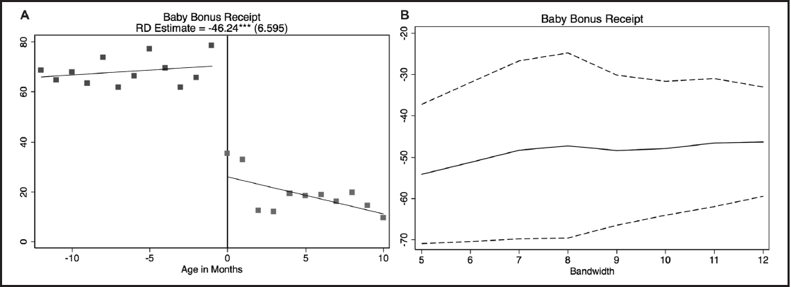
Figure 6
The percentage of mothers receiving the Baby Bonus. (A) Each data point corresponds to the average value of the percentage of mothers receiving the Baby Bonus by month of birth of the child in 1-month bins. The window includes all children born to mothers from January 2010 until November 2011. The vertical line denotes the PPL cutoff of January 1 2011, normalized to 0. (B) The equivalent coefficient estimates and associated 95% confidence intervals when equation 1 is estimated using 3, 4, ..., 12 month-of-birth cohorts on either side of the threshold.
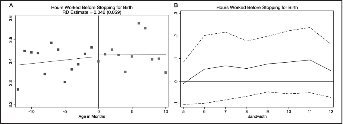
Figure 7
Average number of hours worked by the mother immediately before stopping work for the birth of her child. (A) Each data point corresponds to the average value of each outcome by month of birth of the child in 1-month bins. The window includes all children born to mothers from January 2010 until November 2011. The vertical line denotes the PPL cutoff of January 1 2011, normalized to 0. (B) The equivalent coefficient estimates and associated 95% confidence intervals when equation 1 is estimated using 3, 4, ..., 12 month-of-birth cohorts on either side of the threshold.
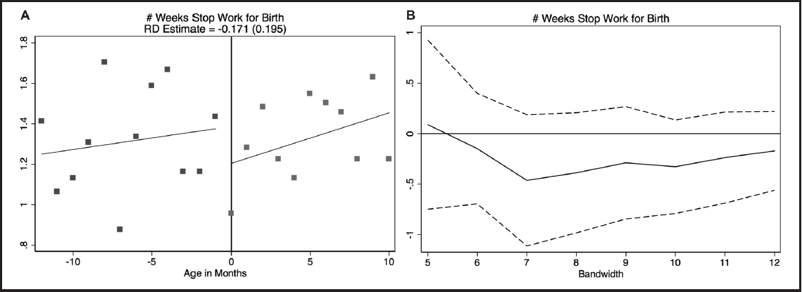
Figure 8
Average number of weeks the mother stopped work before the birth of her child. (A) Each data point corresponds to the average value of each outcome by month of birth of the child in 1-month bins. The window includes all children born to mothers from January 2010 until November 2011. The vertical line denotes the PPL cutoff of January 1 2011, normalized to 0. (B) The equivalent coefficient estimates and associated 95% confidence intervals when equation 1 is estimated using 3, 4, ..., 12 month-of-birth cohorts on either side of the threshold.
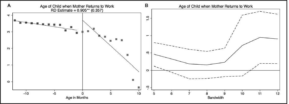
Figure 9
Average age of the child when the mother returned to work. (A) Each data point corresponds to the average value of each outcome by month of birth of the child in 1-month bins. The window includes all children born to mothers from January 2010 until November 2011. The vertical line denotes the PPL cutoff of January 1 2011, normalized to 0. (B) The equivalent coefficient estimates and associated 95% confidence intervals when equation 1 is estimated using 3, 4, ..., 12 month-of-birth cohorts on either side of the threshold.
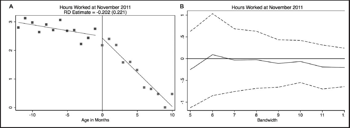
Figure 10
Average number of hours worked by the mother as of November 2011. (A) Each data point corresponds to the average value of each outcome by month of birth of the child in 1-month bins. The window includes all children born to mothers from January 2010 until November 2011. The vertical line denotes the PPL cutoff of January 1 2011, normalized to 0. (B) The equivalent coefficient estimates and associated 95% confidence intervals when equation 1 is estimated using 3, 4, ..., 12 month-of-birth cohorts on either side of the threshold.