
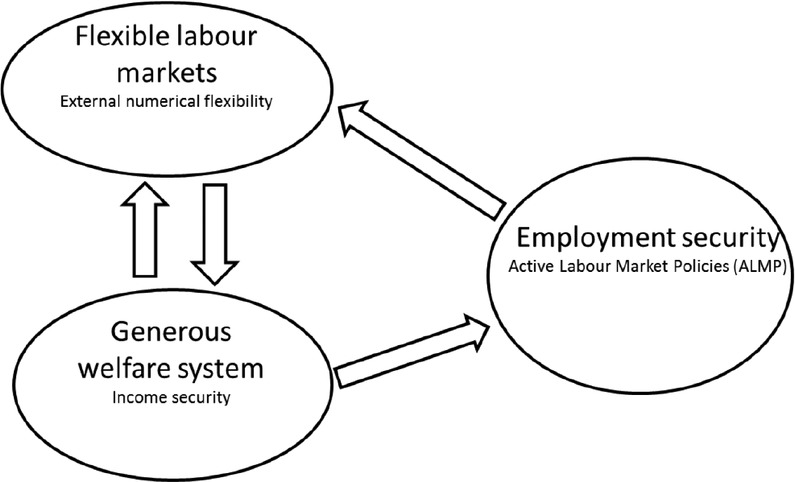
Figure 1
Matrix categories of the Danish golden triangle.
Note: Own elaboration, based on Madsen (1999).
Table 1
Flexibility and security matrix: categories and drivers
| Flexicurity components | Categories | Drivers |
|---|---|---|
| Flexibility | External numerical flexibility | Employment protection legislation (EPL) and tenure |
| Job seekers | ||
| Public expenditure | ||
| Traps | ||
| Family and labor supply | ||
| Low-wage supply | ||
| Transitions | ||
| Internal numerical flexibility | Working time | |
| Functional flexibility | Human capital—lower education | |
| Human capital—higher education, LLL, and ALMP | ||
| Wage flexibility | Competitive pay and labor cost | |
| Security | Job security | EPL and tenure |
| Transitions and self-employment | ||
| Involuntary part-time and temporary jobs | ||
| Employment security | Human capital—lower education | |
| Human capital—higher education, LLL, and ALMP Social security support | ||
| Income security | Social security support | |
| In-work poverty | ||
| Work–life balance | Childcare, parenthood, and inactivity | |
| Part-time and low wage | ||
Table 2
Indicators by flexibility category and driver
| Category and driver | Indicators | Direction |
|---|---|---|
| External numerical flexibility | ||
| F.1. EPL and tenure (F´1) | EPL regular contracts (FRCA_01_r) | − |
| EPL temporary contracts (FRCA_01_t) | − | |
| Job tenure in years—Job duration (FRCA_20) | − | |
| F.2. Job seekers | Unemployment rate (ALMP_02) | + |
| Involuntary working on a temporary job (FRCA_11) | + | |
| Involuntary working part-time (FRCA_12) | + | |
| Diversity and reason for contractual and working arrangements— | + | |
| self-employed (FRCA_14) | ||
| F.3. Public expenditure | Net replacement rate after 6 months (MSS_07) | − |
| PLMP expenditure on support per person in labor reserve (MSS_02) | − | |
| Expenditure on PLMP as % GDP (MSS_03) | − | |
| PLMP participants % of U (MSS_04) | − | |
| F.4. Traps | Unemployment trap (MSS_05) | − |
| Low wage trap (MSS_06) | − | |
| Inactivity trap (WLB_03)1 | − | |
| F.5. Family and labor | Employment impact of parenthood (WLB_04) | − |
| supply | Lack of care for children and other dependents—Main reason for inactivity | − |
| (WLB_07) | ||
| F.6. Low-wage supply | In-work at-risk-of-poverty (TSDSC320) | + |
| At-risk-of-poverty without dependent children no low-work intensity | + | |
| (TESSI122) | ||
| A t-risk-of-poverty with dependent children no low-work intensity (ILC_PEES02) | + | |
| Net replacement rate after 5 years (MSS_08) | − | |
| F.7 Transitions | Transition from temporary to permanent—3-year average (FRCA_04) | − |
| Transition in labor status and pay levels—Same or higher qualification level | + | |
| (CLLL_06)2 | ||
| Internal numerical flexibility | ||
| Working time | <No EMCO indicator> | |
| Functional flexibility | ||
| F.8. Human capital— | Percentage of the population having completed at least secondary | − |
| lower education | education (TPS00065) | |
| At least upper secondary educational attainment, age group 20–24 by sex | + | |
| (TPS00186) | ||
| F.9. Human capital— | LLL (age 25–64) (CLLL_01) | + |
| higher education, LLL, and ALMP | Public spending on human resources (CLLL_02) Educational attainment—% aged 30–34 with tertiary educational attain- | + + |
| ment (CLLL_07) | ||
| Expenditure on ALMP per person in labor service (ALMP_04) | + | |
| Expenditure on ALMP as % GDP (ALMP_05) | + | |
| Activation—LMP participants per 100 persons wanting to work (ALMP_06) | + | |
| Wage flexibility | ||
| F.10. Competitive pay | Transitions by contract—Pay level (FRCA_06) | − |
| and labor cost | ||
[i] 1 Between brackets variables names used in the Annexes. WLB refer to Work Life Balance, CLLL refers to Lifelong Learning and LTU to Long Term Unemployment, FRCA to Flexible and Reliable Contractual Agreements, ALMP to Active Labor Market Policies, and MSS to Modern Social Security (EMCO 2009). Reaming codes are Eurostat codes.
2 Between brackets variables names used in the Annexes. WLB refer to Work Life Balance, CLLL refers to Lifelong Learning and LTU to Long Term Unemployment, FRCA to Flexible and Reliable Contractual Agreements, ALMP to Active Labor Market Policies, MSS to Modern Social Security. Reaming codes are Eurostat codes.
Table 3
Indicators by security category and driver
| Category and driver | Indicators | Direction |
|---|---|---|
| Job security | ||
| S.1. EPL and tenure | EPL regular contracts (FRCA_01_r) | + |
| EPL temporary contracts (FRCA_01_t) | + | |
| Job tenure in years—Job duration (FRCA_20) | + | |
| S.2. Transitions and | Transition from temporary to permanent—3-year average (FRCA_04) | + |
| self-employment | Transitions by contract—Pay level (FRCA_06) | + |
| Diversity and reason for contractual and working arrangements— self-employed (FRCA_14) | − | |
| S.3 Involuntary part-time and temporary jobs | Diversity and reason for contractual and working arrangements—Involuntary part-time (FRCA_12) | − |
| Diversity and reason for contractual and working arrangements—Involuntary temporary (FRCA_11) | − | |
| Employment security | ||
| S.4. Human capital—lower education | Early leavers from education and training (TSDSC410) | − |
| Percentage of the population having completed at least secondary education (TPS00065) | + | |
| At least upper secondary educational attainment, age group 20–24 by sex (TPS00186) | + | |
| S.5. Human capital— | LLL (age 25–64) (CLLL_01) | |
| higher education, LLL, | Public spending on human resources (CLLL_02) | + |
| and ALMP (S´5) | Educational attainment—% aged 30–34 with tertiary educational attainment (CLLL_07) | + |
| Expenditure on ALMP as % GDP (ALMP_05) | + | |
| Activation—LMP participants per 100 persons wanting to work (ALMP_06) | + | |
| Expenditure on ALMP per person in labor service (ALMP_04) | + | |
| LTU 1 (% active population) (ALMP_01) | − | |
| Income security | ||
| S.6. Social security | PLMP expenditure on support per person in labor reserve (MSS_02) | + |
| support | Expenditure on PLMP as % GDP (MSS_03) | + |
| PLMP participants % of U (MSS_04) | + | |
| Net replacement rate after 6 months (MSS_07) | + | |
| Net replacement rate after 5 years (MSS_08) | + | |
| S.7. In-work poverty | At risk of poverty rate max secondary education (TSDSC420) | − |
| In work at risk of poverty (TSDSC320) | − | |
| At risk of poverty without dependent children no low-work intensity (TESSI122) | − | |
| At risk of poverty with dependent children no low-work intensity (ILC_PEES02) | − | |
| Inactivity trap (WLB_03) | + | |
| Work–life balance/combination security | ||
| S.8. Childcare, | Childcare (WLB_02) | + |
| parenthood, and | Employment impact of parenthood (WLB_04) | − |
| inactivity | Lack of care for children and other dependents—the main reason for inactivity (WLB_07) | − |
| S.9. Part-time and low wage | Lack of care for children and other dependents—the main reason for part-time (WLB_06) | − |
| Low wage trap (MSS_06) | − | |
[i] 1 Between brackets variables names used in the Annexes. WLB refer to Work Life Balance, CLLL refers to Lifelong Learning and LTU to Long Term Unemployment, FRCA to Flexible and Reliable Contractual Agreements, ALMP to Active Labor Market Policies, MSS to Modern Social Security. Reaming codes are Eurostat codes.
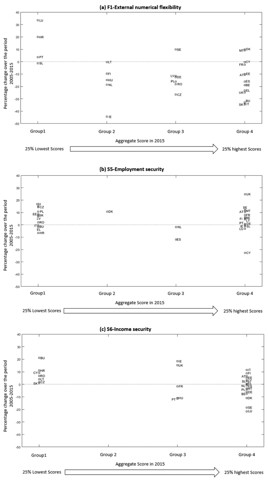
Figure 2
EU-28 performance over 2005–2015 in the golden triangle drivers.
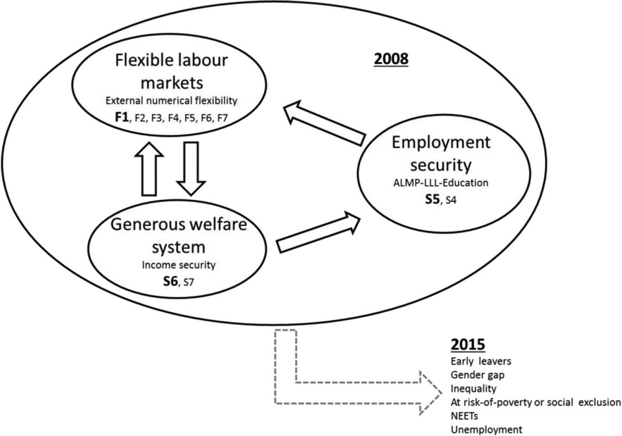
Figure 3
Golden Triangle underlying the linear regression models.
Source: Own elaboration.
Table 4
Explained variables included in the econometric analysis
| Social outcomes (dependent variables) | |||
|---|---|---|---|
| Variable | Concept | Definition | Source |
| Y1 | Early leavers from edu- cation and training | Percentage of the population between 18 and 24-year-old with at most secondary education who were not in further education or training during the last 4 weeks preceding the survey in 2015 | Social Scoreboard for the European Pillar of Social |
| Y2 | Gender gap | Difference between the employment rates of men and women of working age in 2015 | Rights (https:// composite- |
| Y3 | Income inequality | The ratio of total income received by the 20% of the population with the highest income over the income received by the 20% of the population with the lowest levels of income in 2015 | indicators.jrc. ec.europa.eu/ social-scoreboard/) |
| Y4 | At risk of poverty or social exclusion (AROPE) | Percentage of the population who is either at risk of poverty or social exclusion (severely deprived or living in a household with low work intensity in 2015 | |
| Y5 | Young people not in ed- ucation, employment, or training (NEET) | Percentage of young people aged between 15- and 24-year-old who are neither working nor studying or doing a training job in 2015 | |
| Y6 | Unemployment rate | Unemployed people as a percentage of the labor force in 2015 | |
Table 5
Independent variables included in the econometric analysis
| Flexicurity measures and controls (explanatory variables) | ||||||
|---|---|---|---|---|---|---|
| Matrix | Variable | Concept | Definition | Source | ||
| Flexicurity | X | Flexibility | F1 | External nu- merical flexibil- | The aggregated value of the driver “EPL and tenure” in 2008 | Own elaboration |
| ity in the labor | ||||||
| market | ||||||
| S5 | Employment | The aggregated value of the driver | ||||
| Security | security | “Human Capital—higher education, LLL, and ALMP” in 2008 | ||||
| S6 | Income security | The aggregated value of the driver | ||||
| “Social security support” in 2008 | ||||||
| Control | C | L | Lagged depen- dent variable | Value of the dependent variable in 2008 | Social Scoreboard for the European Pillar of Social | |
| Rights | ||||||
| ln(GDP) | GDP per capita | Natural logarithm of GDP per capita in | Eurostat | |||
| 2008 | ||||||
| νGDP | Economic | The annual average growth rate of GDP | ||||
| growth | per capita over the period 2008–2015 | |||||
| Outliers | D | Country dummies | Dummy for each country detected as outlier according to the DFFIT1 analysis | Own elaboration | ||
[i] 1 The definition of DFFITS is “Difference in Fits”. Therefore, the footnote 5 on page 15 (line 42) should start in the following way: “The detection of outliers is based on the Difference in Fits (DFFITS) analysis”.
Table 6
Results of the OLS regression over the period 2008–2015
| Social outcomes | |||||||||
|---|---|---|---|---|---|---|---|---|---|
| Variables | Y1,2015 | Y2,2015 | Y3,2015 | Y4,2015 | Y5,2015 | Y6,2015 | |||
| Constant | 11.479 | −6.677 | 2.192 | −22.675 | 7.589 | 18.015 | |||
| Flexicurity | Flexibility | External numerical | F1,2008 | 0.004 | 0.039 | −0.006 | −0.035* | −0.023 | −0.061* |
| Security | Employment security | S5,2008 | −0.048 | −0.009 | 0.023* | 0.067 | 0.001 | 0.0773 | |
| Income security | S6,2008 | 0.055** | −0.018 | −0.013 | −0.063* | −0.014 | −0.046 | ||
| Control variables | L2008 | 0.553*** | 0.843*** | 1.159*** | 1.021*** | 1.056*** | 0.695*** | ||
| ln_GDP2008 | −0.946 | 0.323 | −0.279 | 2.435 | −0.403 | −1.035 | |||
| νGDP08−15 | 6.200** | 5.613 | −0.348 | −7.904 | −4.549** | −15.781*** | |||
| Diagnostic checking | |||||||||
| Adjusted R2 | 0.91 | 0.88 | 0.86 | 0.87 | 0.83 | 0.83 | |||
| Heterocedasticity | B-P-G test | 0.65 (0.74) | 0.99 (0.47) | 1.329 (0.29) | 0.537 (0.84) | 0.546 (0.79) | 1.399 (0.26) | ||
| White test | 0.753 (0.66) | 0.62 (0.75) | 1.330 (0.29) | 0.449 (0.90) | 0.595 (0.75) | 0.939 (0.52) | |||
| Autocorrelation | LM test | 0.008 (0.93) | 0.41 (0.53) | 0.007 (0.94) | 0.013 (0.91) | 0.653 (0.43) | 0.005 (0.94) | ||
| L-B test | 0.012 (0.91) | 0.51 (0.48) | 0.008 (0.93) | 0.018 (0.89) | 0.630 (0.43) | 0.008 (0.93) | |||
| Normality (Jarque–Bera | test) | 0.581 (0.75) | 0.43 (0.81) | 0.830 (0.66) | 4.437 (0.11) | 0.802 (0.67) | 1.680 (0.43) | ||
| Model specification (Ramsey | Reset | 0.113 (0.91) | 0.42 (0.68) | 0.914 (0.37) | 0.217 (0.83) | 1.110 (0.28) | 1.940* (0.07) | ||
| Test) | |||||||||
[i] *, **, ***Statistically significant at the 10, 5, and 1% levels, respectively.
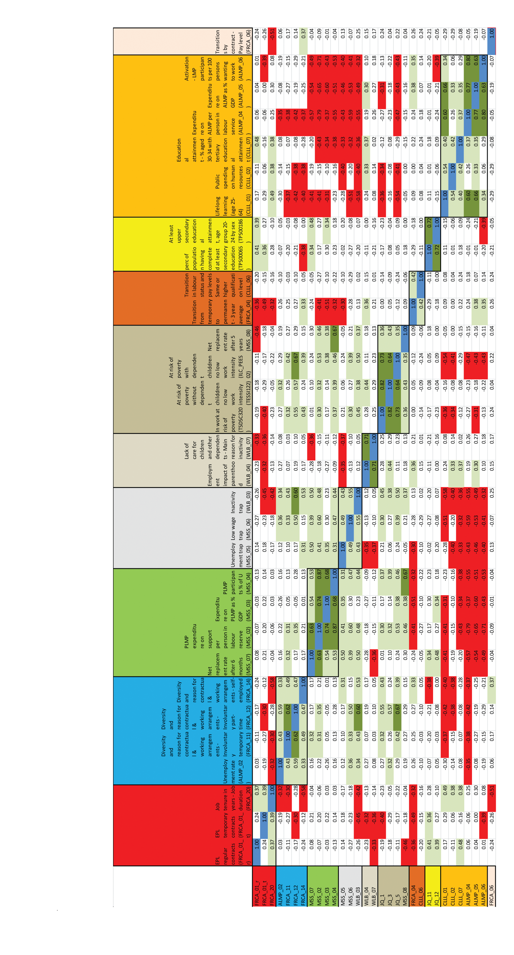
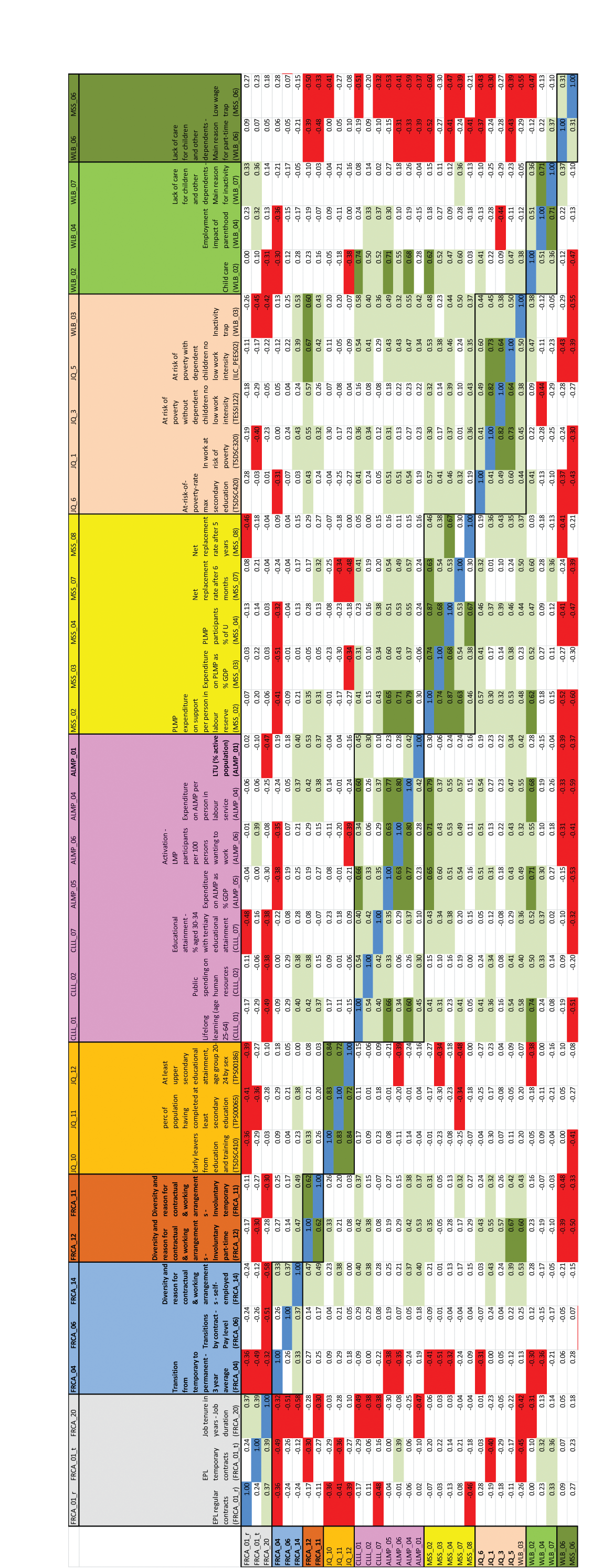
Annex A3
Flexibility drivers—PCA and Cronbach’s α results
| Group 1# FRCA_01_r FRCA_01_t FRCA_20 | ||||||
|---|---|---|---|---|---|---|
| PC1 | PC2 | PC3 | ||||
| SS loadings | 1.673 | 0.757 | 0.570 | |||
| Proportion Var | 0.558 | 0.252 | 0.190 | |||
| Cumulative Var | 0.558 | 0.810 | 1.000 | |||
| Proportion explained | 0.558 | 0.252 | 0.190 | |||
| Cumulative proportion | 0.558 | 0.810 | 1.000 | |||
| Cronbach’s α: 0.61 | ||||||
| Group 2# ALMP_02 FRCA_11 FRCA_12 FRCA_14 | ||||||
| PC1 | PC2 | PC3 | PC4 | |||
| SS loadings | 2.479 | 0.693 | 0.497 | 0.331 | ||
| Proportion Var | 0.620 | 0.173 | 0.124 | 0.083 | ||
| Cumulative Var | 0.620 | 0.793 | 0.917 | 1.000 | ||
| Proportion explained | 0.620 | 0.173 | 0.124 | 0.083 | ||
| Cumulative proportion | 0.620 | 0.793 | 0.917 | 1.000 | ||
| Cronbach’s α: 0.80 | ||||||
| Group 3# MSS_07 MSS_02 MSS_03 MSS_04 | ||||||
| PC1 | PC2 | PC3 | PC4 | |||
| SS loadings | 3.010 | 0.531 | 0.341 | 0.118 | ||
| Proportion Var | 0.752 | 0.133 | 0.085 | 0.030 | ||
| Cumulative Var | 0.752 | 0.885 | 0.970 | 1.000 | ||
| Proportion explained | 0.752 | 0.133 | 0.085 | 0.030 | ||
| Cumulative proportion | 0.752 | 0.885 | 0.970 | 1.000 | ||
| Cronbach’s α: 0.89 | ||||||
| Group 4# MSS_05 MSS_06 WLB_03 | ||||||
| PC1 | PC2 | PC3 | ||||
| SS loadings | 1.989 | 0.577 | 0.434 | |||
| Proportion Var | 0.663 | 0.192 | 0.145 | |||
| Cumulative Var | 0.663 | 0.855 | 1.000 | |||
| Proportion explained | 0.663 | 0.192 | 0.145 | |||
| Cumulative proportion | 0.663 | 0.855 | 1.000 | |||
| Cronbach’s α: 0.70 | ||||||
| Group 6# JQ_1 JQ_3 JQ_5 MSS_08 | ||||||
| PC1 | PC2 | PC3 | PC4 | |||
| SS loadings | 2.713 | 0.755 | 0.373 | 0.160 | ||
| Proportion Var | 0.678 | 0.189 | 0.093 | 0.040 | ||
| Cumulative Var | 0.678 | 0.867 | 0.960 | 1.000 | ||
| Proportion explained | 0.678 | 0.189 | 0.093 | 0.040 | ||
| Cumulative proportion | 0.678 | 0.867 | 0.960 | 1.000 | ||
| Cronbach’s α: 0.83 | ||||||
| Group 9# CLLL_01 CLLL_02 CLLL_07 ALMP_04 ALMP_05 ALMP_06 | ||||||
| PC1 | PC2 | PC3 | PC4 | PC5 | PC6 | |
| SS loadings | 3.359 | 1.200 | 0.674 | 0.383 | 0.240 | 0.144 |
| Proportion Var | 0.560 | 0.200 | 0.112 | 0.064 | 0.040 | 0.024 |
| Cumulative Var | 0.560 | 0.760 | 0.872 | 0.936 | 0.976 | 1.000 |
| Proportion explained | 0.560 | 0.200 | 0.112 | 0.064 | 0.040 | 0.024 |
| Cumulative proportion | 0.560 | 0.760 | 0.872 | 0.936 | 0.976 | 1.000 |
| Cronbach’s α: 0.83 | ||||||
Annex A4
Security drivers—PCA and Cronbach’s α results
| Group 1# FRCA_01_r FRCA_01_t FRCA_20 | |||||||
|---|---|---|---|---|---|---|---|
| PC1 | PC2 | PC3 | |||||
| SS loadings | 1.673 | 0.757 | 0.570 | ||||
| Proportion Var | 0.558 | 0.252 | 0.190 | ||||
| Cumulative Var | 0.558 | 0.810 | 1.000 | ||||
| Proportion explained | 0.558 | 0.252 | 0.190 | ||||
| Cumulative proportion | 0.558 | 0.810 | 1.000 | ||||
| Cronbach’s α: 0.61 | |||||||
| Group 2# FRCA_04 FRCA_06 FRCA_14 | |||||||
| PC1 | PC2 | PC3 | |||||
| SS loadings | 1.641 | 0.746 | 0.613 | ||||
| Proportion Var | 0.547 | 0.249 | 0.204 | ||||
| Cumulative Var | 0.547 | 0.796 | 1.000 | ||||
| Proportion explained | 0.547 | 0.249 | 0.204 | ||||
| Cumulative proportion | 0.547 | 0.796 | 1.000 | ||||
| Cronbach’s α: 0.58 | |||||||
| Group 4# JQ_10 JQ_11 JQ_12 | |||||||
| PC1 | PC2 | PC3 | |||||
| SS loadings | 2.595 | 0.285 | 0.120 | ||||
| Proportion Var | 0.865 | 0.095 | 0.040 | ||||
| Cumulative Var | 0.865 | 0.960 | 1.000 | ||||
| Proportion explained | 0.865 | 0.095 | 0.040 | ||||
| Cumulative proportion | 0.865 | 0.960 | 1.000 | ||||
| Cronbach’s α: 0.92 | |||||||
| Group 5# CLLL_01 CLLL_02 CLLL_07 ALMP_05 ALMP_06 ALMP_04 ALMP_01 | |||||||
| PC1 | PC2 | PC3 | PC4 | PC5 | PC6 | PC7 | |
| SS loadings | 3.575 | 1.206 | 0.918 | 0.590 | 0.378 | 0.191 | 0.141 |
| Proportion Var | 0.511 | 0.172 | 0.131 | 0.084 | 0.054 | 0.027 | 0.020 |
| Cumulative Var | 0.511 | 0.683 | 0.814 | 0.899 | 0.953 | 0.980 | 1.000 |
| Proportion explained | 0.511 | 0.172 | 0.131 | 0.084 | 0.054 | 0.027 | 0.020 |
| Cumulative proportion | 0.511 | 0.683 | 0.814 | 0.899 | 0.953 | 0.980 | 1.000 |
| Cronbach’s α: 0.83 | |||||||
| Group 6# MSS_02 MSS_03 MSS_04 MSS_07 MSS_08 | |||||||
| PC1 | PC2 | PC3 | PC4 | PC5 | |||
| SS loadings | 3.366 | 0.780 | 0.480 | 0.291 | 0.084 | ||
| Proportion Var | 0.673 | 0.156 | 0.096 | 0.058 | 0.017 | ||
| Cumulative Var | 0.673 | 0.829 | 0.925 | 0.983 | 1.000 | ||
| Proportion explained | 0.673 | 0.156 | 0.096 | 0.058 | 0.017 | ||
| Cumulative proportion | 0.673 | 0.829 | 0.925 | 0.983 | 1.000 | ||
| Cronbach’s α: 0.87 | |||||||
| Group 7# JQ_6 JQ_1 JQ_3 JQ_5 WLB_03 | |||||||
| PC1 | PC2 | PC3 | PC4 | PC5 | |||
| SS loadings | 3.214 | 0.746 | 0.575 | 0.326 | 0.139 | ||
| Proportion Var | 0.643 | 0.149 | 0.115 | 0.065 | 0.028 | ||
| Cumulative Var | 0.643 | 0.792 | 0.907 | 0.972 | 1.000 | ||
| Proportion explained | 0.643 | 0.149 | 0.115 | 0.065 | 0.028 | ||
| Cumulative proportion | 0.643 | 0.792 | 0.907 | 0.972 | 1.000 | ||
| Cronbach’s α: 0.85 | |||||||
| Group 8# WLB_02 WLB_04 WLB_07 | |||||||
| PC1 | PC2 | PC3 | |||||
| SS loadings | 2.064 | 0.666 | 0.270 | ||||
| Proportion Var | 0.688 | 0.222 | 0.090 | ||||
| Cumulative Var | 0.688 | 0.910 | 1.000 | ||||
| Proportion explained | 0.688 | 0.222 | 0.090 | ||||
| Cumulative proportion | 0.688 | 0.910 | 1.000 | ||||
| Cronbach’s α: 0.76 | |||||||