
Table 1
Descriptive Statistics
| Earning regression sample | Employment regression sample | |||||
|---|---|---|---|---|---|---|
| N | Mean | SD | N | Mean | SD | |
| Log earnings | 104,577 | 9.656 | 0.738 | - | - | - |
| Employment | - | - | - | 129,966 | 0.919 | 0.273 |
| Isolation index | 8,149 | 0.014 | 0.021 | 8,874 | 0.014 | 0.020 |
| Group average education | 8,149 | 13.136 | 2.241 | 8,874 | 13.153 | 2.241 |
| Immigrant share | 8,149 | 0.004 | 0.015 | 8,874 | 0.004 | 0.014 |
| Education | 104,577 | 11.023 | 4.170 | 129,966 | 10.922 | 4.218 |
| Age | 104,577 | 26.395 | 2.829 | 129,966 | 26.330 | 2.874 |
| Male | 104,577 | 0.680 | 0.467 | 129,966 | 0.655 | 0.475 |
| Married | 104,577 | 0.383 | 0.486 | 129,966 | 0.385 | 0.486 |
| Have children | 104,577 | 0.301 | 0.459 | 129,966 | 0.305 | 0.461 |
| White | 104,577 | 0.121 | 0.326 | 129,966 | 0.121 | 0.326 |
| Black | 104,577 | 0.025 | 0.157 | 129,966 | 0.026 | 0.159 |
| Asian | 104,577 | 0.182 | 0.386 | 129,966 | 0.176 | 0.381 |
| Hispanic | 104,577 | 0.672 | 0.469 | 129,966 | 0.677 | 0.468 |
Table 2
Balancing Tests, Triple Differences Model
| Dependent Variable: Isolation Index × 1000 | ||
|---|---|---|
| (1) | (2) | |
| Education | −0.007 (0.007) | 0.042 (0.060) |
| Age | −0.006 (0.006) | 0.014 (0.021) |
| Male | 0.053 (0.042) | 0.144 (0.127) |
| Black | −0.285 (0.313) | −0.000 (0.870) |
| Other Nonwhite | 0.088 (0.215) | −0.026 (0.395) |
| Age × Education | - | −0.002 (0.002) |
| Male × Education | - | −0.008 (0.011) |
| Black × Education | - | −0.022 (0.060) |
| Other Nonwhite × Education | - | 0.009 (0.027) |
| F-test | 1.05 | 0.45 |
| P-value | 0.385 | 0.771 |
| N | 102,475 | |
[i] Notes: The isolation index is inflated by 1000. We use the sample of immigrants who are from age group 20–30 and arrived at the U.S. after age 17 or later. Figures in parentheses are standard errors robust to clustering at the MSA by country of origin level. The values of F-statistic in column 1 are for the joint effect of all the individual characteristics that are included in the regressions. The values of F-statistic in column 2 are for the joint effect of all the interaction terms. We use STATA command reghdfe (high dimensional fixed effects) to estimate the parameters. The sample size becomes slightly smaller since singleton observations are dropped.
[ii] Significance is defined as follows: ***p<0.01; **p<0.05; *p<0.10.
Table 3
Triple differences, ISO Model and Model, Earnings Results
| Dependent variable: log earning | ||||||
|---|---|---|---|---|---|---|
| (1) | (2) | (3) | (4) | (5) | (6) | |
| ISO | −0.217 (0.469) | −0.233 (0.436) | −0.156 (0.417) | 0.438 (1.721) | −0.498 (1.599) | −0.582 (1.556) |
| - | - | - | −0.039 (0.187) | 0.059 (0.175) | 0.061 (0.170) | |
| - | - | - | 0.055*** (0.013) | 0.049*** (0.012) | 0.023* (0.012) | |
| S | - | - | 0.028*** (0.002) | - | - | 0.028*** (0.002) |
| +characteristic control | No | Yes | Yes | No | Yes | Yes |
| F-test | - | - | - | 0.04 | 0.06 | 0.07 |
| P-value | - | - | - | 0.960 | 0.943 | 0.933 |
| N | 102,475 | |||||
Notes: We use the sample of immigrants who are from age group 20–30 and arrived at the U.S. after age 17 or later. We control for MSA-specific time trends, MSA-specific group effects, and group-specific time trends in all regressions. Characteristic controls include age, gender, marital status, children in the household, black, Asian, and Hispanic dummy variables. The values of F-statistic are for the joint effect of the isolation index and the interaction term between isolation index and group average education. We use STATA command reghdfe (high dimensional fixed effects) to estimate the parameters. The sample size becomes slightly smaller since singleton observations are dropped. Figures in parentheses are standard errors robust to clustering at the MSA by country of origin level.
Significance is defined as follows:
Table 4
Triple Differences and Triple Interactions Model (Centered), Earnings Results
| Dependent variable: log earning | ||||
|---|---|---|---|---|
| (1) | (2) | (3) | (4) | |
| ISO | −0.136 (0.414) | 0.375 (0.846) | 0.415 (0.847) | 0.327 (0.837) |
| ISO × S | −0.174*** (0.021) | −0.029 (0.023) | −0.160* (0.083) | −0.216** (0.096) |
| - | 0.109 (0.169) | 0.117 (0.169) | 0.098 (0.168) | |
| - | - | −0.036* (0.184) | - | |
| - | - | - | 0.505*** (0.138) | |
| - | - | - | −0.048** (0.021) | |
| - | 0.010*** (0.001) | 0.011*** (0.001) | 0.011*** (0.001) | |
| - | 0.007 (0.012) | 0.006 (0.012) | 0.007 (0.012) | |
| S | 0.040*** (0.002) | 0.063*** (0.002) | 0.066*** (0.002) | 0.065*** (0.002) |
| F-test | 33.97 | 0.69 | 1.10 | 3.09 |
| P-value | 0.000 | 0.559 | 0.354 | 0.009 |
| N | 102,475 | |||
Notes: We use the sample of immigrants who are from age group 20–30 and arrived at the U.S. after age 17 or later. To center the variables, we replace ISOgmt, , and Sigmt by , , and , respectively. is equal to is greater than its MSA-year mean, and 0 otherwise. Similarly, is equal to is lower than its MSA-year mean, and 0 otherwise. The values of the F-statistic are for the joint effect of the isolation index and all the interaction terms, except for . Control variables include age, male dummy, whether married, whether have children in the household, black, Asian, Hispanic, group average education (centered), and immigrants’ own education (centered). We use STATA command reghdfe (high dimensional fixed effects) to estimate the parameters. The sample size becomes slightly smaller since singleton observations are dropped. Figures in parentheses are standard errors robust to clustering at the MSA by country of origin level.
Significance is defined as follows:
Table 5
Robustness Tests, Triple Differences and Triple Interactions Model (Centered)
| Dependent variable: log earning | ||||
|---|---|---|---|---|
| (1) | (2) | (3) | (4) | |
| Male | Female | Arrived at the U.S. after age 21 or later | Arrived at the U.S. after age 23 or later | |
| ISO | −0.945 (1.146) | 1.962 (1.618) | −0.572 (1.001) | 0.294 (1.262) |
| ISO × S | −0.281*** (0.095) | −0.108 (0.082) | −0.179 (0.115) | −0.158 (0.129) |
| −0.124 (0.221) | 0.449 (0.329) | −0.187 (0.212) | 0.115 (0.281) | |
| 0.554*** (0.156) | 0.439* (0.233) | 0.513*** (0.183) | 0.368* (0.222) | |
| −0.060*** (0.021) | −0.035* (0.020) | −0.038 (0.025) | −0.033 (0.029) | |
| 0.010*** (0.001) | 0.012*** (0.001) | 0.010*** (0.001) | 0.009*** (0.001) | |
| −0.011 (0.015) | 0.014 (0.025) | −0.001 (0.019) | −0.010 (0.025) | |
| S | 0.060*** (0.003) | 0.071*** (0.003) | 0.065*** (0.003) | 0.063*** (0.003) |
| F-test | 3.68 | 1.88 | 1.73 | 0.73 |
| P-value | 0.003 | 0.095 | 0.123 | 0.600 |
| N | 69,166 | 31,718 | 51,828 | 32,188 |
Notes: To center the variables, we replace ISOgmt, , and Sigmt by , , and , respectively. Control variables include age, male dummy, whether married, whether have children in the household, black, Asian, Hispanic, group average education (centered), and immigrants’ own education (centered). The values of the F-statistic are for the joint effect of the isolation index and all the interaction terms, except for . We use STATA command reghdfe (high dimensional fixed effects) to estimate the parameters. Figures in parentheses are standard errors robust to clustering at the MSA by country of origin level.
Significance is defined as follows:
Table 6
Balancing Tests with Assimilation Measures, Triple Differences Model
| Dependent Variable: Isolation Index × 1000 | ||
|---|---|---|
| (1) | (2) | |
| Education | −0.011 (0.007) | 0.017 (0.061) |
| Age | −0.002 (0.008) | 0.008 (0.023) |
| Male | 0.051 (0.042) | 0.142 (0.129) |
| Black | −0.278 (0.313) | −0.051 (0.867) |
| Other Nonwhite | 0.097 (0.215) | 0.023 (0.409) |
| English Insufficiency | −0.132*** (0.050) | −0.255* (0.154) |
| Years in the U.S. | −0.012 (0.008) | 0.007 (0.019) |
| Age × Education | - | −0.001 (0.002) |
| Male × Education | - | −0.008 (0.011) |
| Black × Education | - | −0.017 (0.060) |
| Other Nonwhite × Education | - | 0.006 (0.028) |
| English Insufficiency × Education | - | 0.012 (0.014) |
| Years in the U.S. × Education | - | −0.002 (0.002) |
| F-test | 1.73 | 0.064 |
| P-value | 0.097 | 0.695 |
| N | 102,475 | |
Notes: The isolation index is inflated by 1000. We use the sample of immigrants who are from age group 20–30 and arrived at the U.S. after age 17 or later. Figures in parentheses are standard errors robust to clustering at the MSA by country of origin level. The values of F-statistic in column 1 are for the joint effect of all the individual characteristics that are included in the regressions. The values of F-statistic in column 2 are for the joint effect of all the interaction terms. We use STATA command reghdfe (high dimensional fixed effects) to estimate the parameters. The sample size becomes slightly smaller since singleton observations are dropped.
Significance is defined as follows:
Table 7
Mechanisms and Heterogeneity Tests, Earning Results
| Dependent variable: log earning | |||
|---|---|---|---|
| Baseline | English insufficiency | Years in the U.S. | |
| ISO | 0.327 (0.837) | 0.320 (0.843) | 0.673 (0.809) |
| ISO × S | −0.216** (0.096) | −0.247*** (0.090) | −0.244*** (0.094) |
| 0.098 (0.168) | 0.132 (0.171) | 0.115 (0.164) | |
| 0.505*** (0.138) | 0.516*** (0.139) | 0.544*** (0.141) | |
| −0.048** (0.021) | −0.056*** (0.020) | −0.057*** (0.021) | |
| insufEng | −0.183*** (0.012) | - | |
| ISO × insufEng | - | 0.046 (0.131) | - |
| Years in US | - | 0.037*** (0.002) | |
| ISO × Years in US | - | - | −0.041** (0.017) |
| F-test | 3.09 | 3.69 | 3.85 |
| P-value | 0.009 | 0.003 | 0.002 |
| N | 102,475 | ||
Notes: To center the variables, we replace ISOgmt, , and Sigmt by , , and , respectively. The values of the F-statistic are for the joint effect of the isolation index and all the interaction terms, except for . Control variables include age, male dummy, whether married, whether have children in the household, black, Asian, Hispanic, group average education (centered), and immigrants’ own education (centered). We use STATA command reghdfe (high dimensional fixed effects) to estimate the parameters. Therefore, singleton observations are dropped. Figures in parentheses are standard errors robust to clustering at the MSA by country of origin level.
Significance is defined as follows:
Table 8
Triple differences, ISO Model and Model, Employment Results
| Dependent variable: if employed, =1 | ||||||
|---|---|---|---|---|---|---|
| (1) | (2) | (3) | (4) | (5) | (6) | |
| ISO | −0.106 (0.151) | −0.109 (0.152) | −0.092 (0.153) | 0.014 (0.514) | −0.061 (0.512) | −0.068 (0.512) |
| - | - | - | −0.014 (0.050) | −0.006 (0.050) | −0.005 (0.050) | |
| - | - | - | −0.001 (0.005) | −0.001 (0.005) | −0.004 (0.005) | |
| S | - | - | 0.003*** (0.000) | - | - | 0.003*** (0.000) |
| +characteristic control | No | Yes | Yes | No | Yes | Yes |
| +individual education control | No | No | Yes | No | No | Yes |
| F-test | - | - | - | 0.37 | 0.31 | 0.31 |
| P-value | - | - | - | 0.690 | 0.736 | 0.736 |
| N | 127,769 | |||||
Notes: We use the sample of immigrants who are from age group 20–30 and arrived at the U.S. after age 17 or later. We control for MSA-specific time trends, MSA-specific group effects, and group-specific time trends in all regressions. Characteristic controls include age, gender, marital status, children in the household, black, Asian, and Hispanic dummy variables. The values of the F-statistic are for the joint effect of the isolation index and the interaction term between isolation index and group average education. We use STATA command reghdfe (high dimensional fixed effects) to estimate the parameters. Therefore, singleton observations are dropped. Figures in parentheses are standard errors robust to clustering at the MSA by country of origin level.
Significance is defined as follows:
Table 9
Triple Differences and Triple Interactions Model (Centered), Employment Results
| Dependent variable: if employed, =1 | ||||
|---|---|---|---|---|
| (1) | (2) | (3) | (4) | |
| ISO | −0.089 (0.153) | −0.009 (0.249) | −0.012 (0.249) | −0.018 (0.249) |
| ISO × S | −0.013** (0.005) | −0.005 (0.006) | 0.005 (0.017) | 0.001 (0.018) |
| - | 0.027 (0.056) | 0.026 (0.056) | 0.025 (0.056) | |
| - | - | 0.003 (0.004) | - | |
| - | - | - | 0.042 (0.037) | |
| - | - | - | 0.002 (0.004) | |
| - | 0.001*** (0.000) | 0.000** (0.000) | 0.000** (0.000) | |
| - | −0.005 (0.004) | −0.005 (0.004) | −0.005 (0.004) | |
| S | 0.004*** (0.000) | 0.005*** (0.001) | 0.005*** (0.001) | 0.005*** (0.001) |
| F-test | 2.97 | 0.49 | 0.57 | 0.68 |
| P-value | 0.052 | 0.687 | 0.686 | 0.635 |
| N | 127,769 | |||
Notes: We use the sample of immigrants who are from age group 20–30 and arrived at the U.S. after age 17 or later. To center the variables, we replace ISOgmt, , and Sigmt by , and , respectively. is equal to is greater than its MSA-year mean, and 0 otherwise. Similarly, is equal to is lower than its MSA-year mean, and 0 otherwise. The values of the F-statistic are for the joint effect of the isolation index and all the interaction terms, except for . Control variables include age, male dummy, whether married, whether have children in the household, black, Asian, Hispanic, group average education (centered), and immigrants’ own education (centered). We use STATA command reghdfe (high dimensional fixed effects) to estimate the parameters. Therefore, singleton observations are dropped. Figures in parentheses are standard errors robust to clustering at the MSA by country of origin level.
Significance is defined as follows:
Table 10
Robustness Test, Triple Differences and Triple Interactions Model (Centered), Employment Results
| Dependent variable: if employed, =1 | ||||
|---|---|---|---|---|
| (1) | (2) | (3) | (4) | |
| Male | Female | Arrived at the U.S. after age 21 or later | Arrived at the U.S. after age 23 or later | |
| ISO | 0.134 (0.304) | −0.346 (0.464) | −0.119 (0.280) | −0.133 (0.332) |
| ISO × S | −0.004 (0.016) | −0.001 (0.029) | 0.039** (0.018) | 0.030 (0.019) |
| 0.038 (0.065) | 0.006 (0.113) | 0.013 (0.069) | 0.115 (0.077) | |
| 0.034 (0.046) | 0.068 (0.057) | 0.036 (0.051) | 0.029 (0.065) | |
| 0.001 (0.004) | −0.001 (0.007) | 0.009** (0.004) | 0.007 (0.005) | |
| 0.001*** (0.000) | −0.001 (0.000) | 0.001** (0.000) | 0.000 (0.000) | |
| −0.005 (0.005) | −0.007 (0.009) | −0.009 (0.006) | −0.011 (0.007) | |
| S | 0.005*** (0.001) | 0.004*** (0.001) | 0.005*** (0.001) | 0.005*** (0.001) |
| F-test | 0.67 | 0.62 | 1.41 | 2.09 |
| P-value | 0.647 | 0.686 | 0.219 | 0.063 |
| N | 83,164 | 42,838 | 65,149 | 40,642 |
Notes: The sample used for robustness test is restricted to immigrants who arrived at the U.S. after age 21 or 23. To center the variables, we replace ISOgmt, , and Sigmt by , , and , respectively. Control variables include age, male dummy, whether married, whether have children in the household, black, Asian, Hispanic, group average education (centered), and immigrants’ own education (centered). The values of the F-statistic are for the joint effect of the isolation index and all the interaction terms, except for . We use STATA command reghdfe (high dimensional fixed effects) to estimate the parameters. Therefore, singleton observations are dropped. Figures in parentheses are standard errors robust to clustering at the MSA by country of origin level.
Significance is defined as follows:
Table 11
Mechanisms and Heterogeneity Tests, Employment Results
| Dependent variable: if employed, =1 | |||
|---|---|---|---|
| Baseline | English insufficiency | Years in the U.S. | |
| ISO | −0.018 (0.249) | −0.028 (0.249) | 0.024 (0.251) |
| ISO × S | 0.001 (0.018) | −0.000 (0.018) | −0.001 (0.018) |
| 0.025 (0.056) | 0.031 (0.056) | 0.027 (0.056) | |
| 0.042 (0.037) | 0.042 (0.037) | 0.043 (0.038) | |
| 0.002 (0.004) | 0.001 (0.004) | 0.001 (0.004) | |
| ISO × insufEng | - | 0.045 (0.043) | - |
| insufEng | - | −0.021*** (0.004) | - |
| ISO × Years in US | - | - | −0.006 (0.007) |
| Years in US | - | - | 0.003*** (0.001) |
| F-test | 0.68 | 0.65 | 0.57 |
| P-value | 0.635 | 0.664 | 0.721 |
| N | 127,769 | ||
Notes: To center the variables, we replace ISOgmt, , and Sigmt by , , and , respectively. The values of the F-statistic are for the joint effect of the isolation index and all the interaction terms, except for . Control variables include age, male dummy, whether married, whether have children in the household, black, Asian, Hispanic, group average education (centered), and immigrants’ own education (centered). We use STATA command reghdfe (high dimensional fixed effects) to estimate the parameters. Therefore, singleton observations are dropped. Figures in parentheses are standard errors robust to clustering at the MSA by country of origin level.
Significance is defined as follows:
Table A.1
Cutler et al. (2008) Model, Earning Results
| Dependent Var: log earning | ISO Model | ISO, Model | ||||
|---|---|---|---|---|---|---|
| (1) | (2) | (3) | (4) | |||
| OLS+FE | IV | OLS+FE | IV | |||
| ISO | ISO | ISO | ISO | |||
| Cutler et al. (2007) | 0.250 (0.512) | 2.963** (1.525) | 2.965* (1.600) | −0.331* (0.183) | −14.021*** (5.212) | 1.637*** (0.568) |
| N | 22,564 | 22,564 | 22,564 | 22,564 | ||
| 2000, 60 groups (age 20–30) | −0.280** (0.142) | 1.557 (0.971) | −2.034 (5.157) | 0.229 (0.356) | −3.977 (3.118) | 0.361 (0.221) |
| N | 97,861 | |||||
| 2010, 74 groups (age 20–30) | 0.256* (0.143) | 1.048 (0.703) | −0.425 (0.547) | 0.062 (0.049) | 5.618 (8.350) | −0.319 (0.596) |
| N | 98,672 | |||||
| 2000, 60 groups (age 20–30, arrived after age 17) | −0.361* (0.187) | −0.308 (1.667) | 1.300* (0.723) | −0.162** (0.067) | 132.097 (4536.585) | −8.553 (293.454) |
| N | 53,690 | |||||
| 2010, 74 groups (age 20–30, arrived after age 17) | 0.304 (0.203) | −0.277 (0.988) | 0.051 (0.767) | 0.023 (0.070) | 36.310 (105.392) | −2.641 (7.558) |
| N | 51,994 | |||||
Notes: We control for MSA and country of origin fixed effects in the OLS model. All the control variables are the same as models in Cutler et al. (2008). The instrumental variable used for IV estimation is mean years of ethnic group g in MSA s since immigration. Figures in parentheses are standard errors robust to clustering at the MSA by country of origin level.
Significance is defined as follows:
Table A.2
Balancing Tests for Isolation Index and Cutler et al. (2007) Instrument Variable
| Dependent Variable: | Isolation Index × 1000 | Mean Years of Immigrant Group g in MSA s since immigration | ||
|---|---|---|---|---|
| (1) | (2) | (3) | (4) | |
| 2000 | 2010 | 2000 | 2010 | |
| Education | −0.663*** (0.137) | −0.466*** (0.110) | 0.002 (0.005) | 0.007 (0.005) |
| Age | −0.037 (0.056) | 0.072 (0.046) | 0.020*** (0.005) | 0.021*** (0.004) |
| Male | −0.518 (0.343) | −0.315 (0.357) | −0.103*** (0.029) | −0.157*** (0.031) |
| Black | 1.573 (2.385) | −1.077 (2.571) | −0.113 (0.270) | −0.209 (0.355) |
| Other Nonwhite | −1.177 (1.325) | 1.382 (1.497) | −0.370** (0.157) | −0.530** (0.197) |
| F-test | 6.48 | 4.07 | 6.71 | 10.53 |
| P-value | 0.000 | 0.001 | 0.000 | 0.000 |
| N | 53,690 | 51,994 | 53,690 | 51,994 |
Notes: Sample is restricted to immigrants who are from age group 20–30 and arrived at the U.S. after age 17 or later. MSA and country of origin fixed effects are included in all the regressions. The isolation index is inflated by 1000. Figures in parentheses are standard errors robust to clustering at the MSA by country of origin level. The F-statistic is for the joint effect of all the individual characteristics that are included in the regressions.
Significance is defined as follows:
Table A.3
Balancing Tests, MSA and Group Fixed Effects vs. Triple Differences Model
| Panel 1. Dependent Variable: Isolation Index × 1000 | ||||
|---|---|---|---|---|
| MSA FE, Group FE | Triple Differences | |||
| Education | −0.607*** (0.108) | −0.171 (0.449) | −0.007 (0.007) | 0.042 (0.060) |
| Age | 0.006 (0.061) | 0.402** (0.196) | −0.006 (0.006) | 0.014 (0.021) |
| Male | −0.637** (0.290) | −3.671*** (1.239) | 0.053 (0.042) | 0.144 (0.127) |
| Black | 1.682 (1.793) | 1.804 (5.049) | −0.285 (0.313) | −0.000 (0.870) |
| Other Nonwhite | 0.506 (1.047) | −4.596 (3.064) | 0.088 (0.215) | −0.026 (0.395) |
| Age × Education | - | −0.038** (0.017) | - | −0.002 (0.002) |
| Male × Education | - | 0.262** (0.109) | - | −0.008 (0.011) |
| Black × Education | −0.028 (0.342) | - | −0.022 (0.060) | |
| Other Nonwhite × Education | - | 0.392* (0.210) | - | 0.009 (0.027) |
| F-test | 7.76 | 6.26 | 1.05 | 0.45 |
| P-value | 0.000 | 0.000 | 0.385 | 0.771 |
| N | 104,555 | 102,475 | ||
| Panel 2. Dependent Variable: Mean Years of Immigrant Group g in MSA s since immigration | ||||
|---|---|---|---|---|
| MSA FE, Group FE | Triple Differences | |||
| Education | 0.040*** (0.006) | 0.206*** (0.037) | 0.002** (0.001) | −0.010 (0.009) |
| Age | 0.052*** (0.005) | 0.100*** (0.010) | 0.002** (0.001) | −0.002 (0.002) |
| Male | −0.155*** (0.028) | 0.074 (0.064) | −0.006 (0.005) | 0.006 (0.013) |
| Black | −0.022 (0.264) | −0.534 (0.609) | −0.002 (0.057) | −0.107 (0.126) |
| Other Nonwhite | −0.178 (0.141) | 0.228 (0.395) | −0.012 (0.039) | −0.028 (0.086) |
| Age × Education | - | −0.005*** (0.001) | - | 0.000** (0.000) |
| Male × Education | - | −0.020*** (0.006) | - | −0.001 (0.001) |
| Black × Education | - | 0.040 (0.043) | - | 0.008 (0.008) |
| Other Nonwhite × Education | - | −0.031 (0.028) | - | 0.001 (0.006) |
| F-test | 39.86 | 11.77 | 2.80 | 1.58 |
| P-value | 0.000 | 0.000 | 0.016 | 0.178 |
| N | 104,555 | 102,475 | ||
Notes: The isolation index is inflated by 1000. The sample is restricted to immigrants who are from age group 20–30 and arrived at the U.S. after age 17 or later. Figures in parentheses are standard errors robust to clustering at the MSA by country of origin level. The values of F-statistic in column 1 and 3 are for the joint effect of all the individual characteristics that are included in the regressions. The values of F-statistic in column 2 and 4 are for the joint effect of all the interaction terms. We use STATA command reghdfe (high dimensional fixed effects) to estimate the parameters. Therefore, singleton observations are dropped in the triple differences model.
Significance is defined as follows:
Table A.4
Additional Robustness Tests Results
| Dependent variable: log earning | ||||||
|---|---|---|---|---|---|---|
| Baseline | Drop blacks | Drop English speakers | ||||
| ISO | 0.415 (0.847) | 0.327 (0.837) | 0.656 (0.863) | 0.558 (0.852) | 1.401 (0.904) | 1.324 (0.893) |
| ISO × S | −0.160* (0.083) | −0.216** (0.096) | −0.174** (0.087) | −0.235** (0.103) | −0.178** (0.086) | −0.227** (0.098) |
| 0.117 (0.169) | 0.098 (0.168) | 0.147 (0.171) | 0.127 (0.170) | 0.359** (0.176) | 0.344** (0.174) | |
| −0.036* (0.018) | - | −0.039** (0.019) | - | −0.041** (0.019) | - | |
| - | 0.505*** (0.138) | - | 0.546*** (0.142) | - | 0.511*** (0.143) | |
| - | −0.048** (0.021) | - | −0.052** (0.022) | - | −0.051** (0.022) | |
| F-test | 1.10 | 3.09 | 1.24 | 3.39 | 2.32 | 4.03 |
| P-value | 0.354 | 0.009 | 0.293 | 0.005 | 0.055 | 0.001 |
| N | 102,475 | 99,939 | 93,251 | |||
| Dependent variable: if employed, =1 | ||||||
|---|---|---|---|---|---|---|
| Baseline | Drop blacks | Drop English speakers | ||||
| ISO | −0.012 (0.249) | −0.018 (0.249) | −0.097 (0.247) | −0.104 (0.247) | 0.023 (0.261) | 0.020 (0.261) |
| ISO × S | 0.005 (0.017) | −0.001 (0.018) | 0.002 (0.017) | −0.003 (0.018) | 0.007 (0.017) | 0.005 (0.017) |
| 0.026 (0.056) | 0.025 (0.056) | 0.015 (0.055) | 0.014 (0.055) | 0.039 (0.059) | 0.038 (0.059) | |
| 0.003 (0.004) | - | 0.002 (0.004) | - | 0.004 (0.004) | - | |
| - | 0.042 (0.037) | - | 0.047 (0.038) | - | 0.024 (0.034) | |
| - | 0.002 (0.004) | - | 0.001 (0.004) | - | 0.003 (0.004) | |
| F-test | 0.57 | 0.68 | 0.59 | 0.74 | 0.76 | 0.69 |
| P-value | 0.686 | 0.635 | 0.672 | 0.590 | 0.552 | 0.633 |
| N | 127,769 | 124,480 | 116,493 | |||
Notes: To center the variables, we replace ISOgmt, , and Sigmt by , , and , respectively. The values of the F-statistic are for the joint effect of the isolation index and all the interaction terms, except for . We use STATA command reghdfe (high dimensional fixed effects) to estimate the parameters. Therefore, singleton observations are dropped. Figures in parentheses are standard errors robust to clustering at the MSA by country of origin level.
Significance is defined as follows:
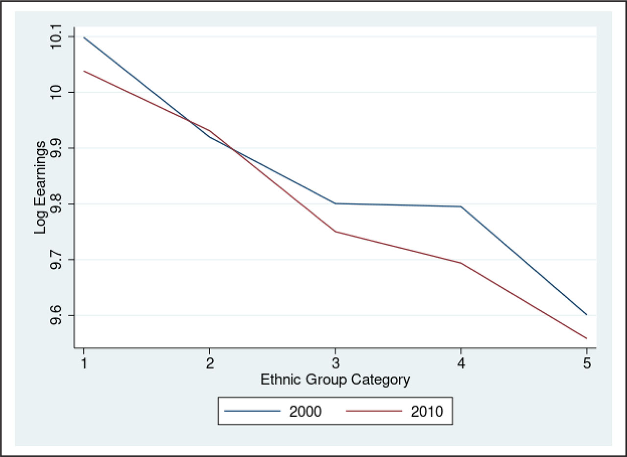
Figure B.1
Differences-in-Differences Trends, Method 1.
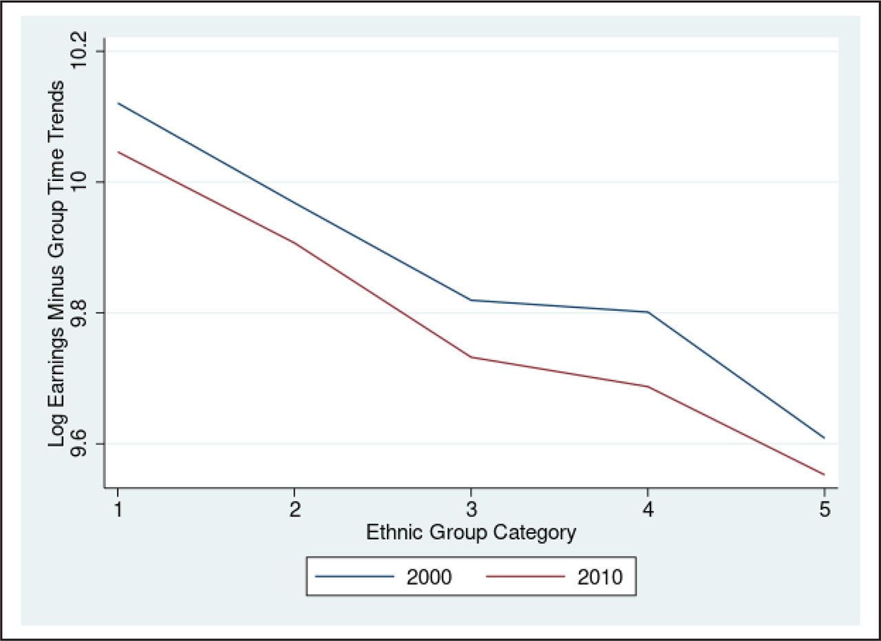
Figure B.2
Triple Differences Trends, Method 1.
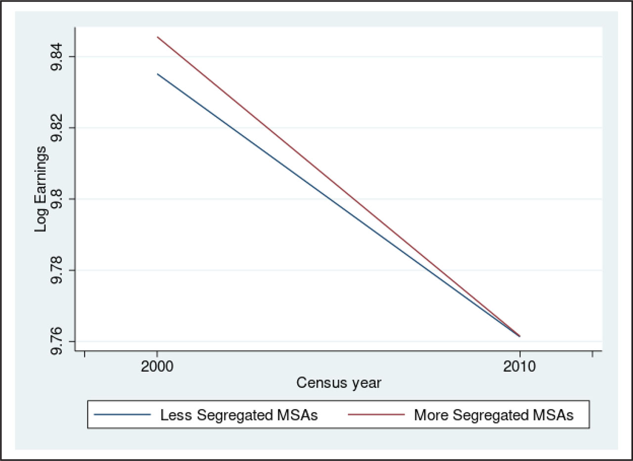
Figure B.3
Differences-in-Differences Trends, Method 2.
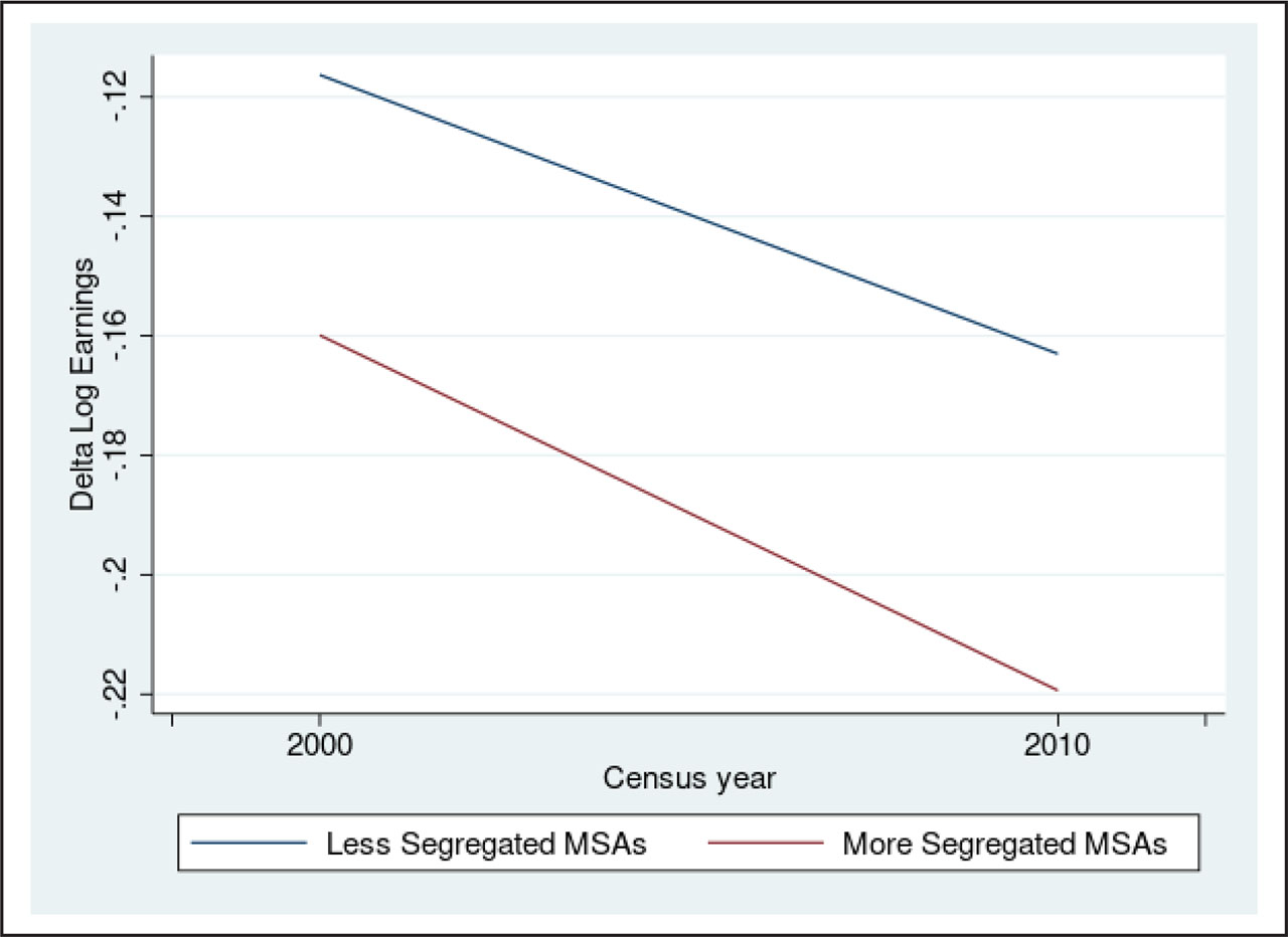
Figure B.4
Triple Differences Trends, Method 2.
Table C.1
Discrete Education Measure, Triple differences, ISO Model and Model
| Dependent variable: log earning | ||||||
|---|---|---|---|---|---|---|
| (1) | (2) | (3) | (4) | (5) | (6) | |
| ISO | −0.217 (0.469) | −0.233 (0.436) | −0.136 (0.416) | −1.074 (1.047) | −1.044 (0.963) | −1.142 (0.934) |
| ISO × %HS | - | - | - | 3.608 (3.381) | 3.122 (3.084) | 3.181 (3.030) |
| ISO × %Some_Coll | - | - | - | 2.358 (5.551) | −0.283 (5.207) | −0.780 (4.869) |
| ISO × %College | - | - | - | −0.040 (2.317) | 1.427 (2.190) | 2.001 (2.075) |
| %High School | - | - | - | −0.158 (0.130) | −0.145 (0.124) | −0.210* (0.122) |
| %Some College | - | - | - | 0.042 (0.167) | 0.079 (0.158) | −0.068 (0.154) |
| %College | - | - | - | 0.651*** (0.142) | 0.559*** (0.134) | 0.139 (0.131) |
| High School | - | - | 0.090*** (0.006) | - | - | 0.090*** (0.006) |
| Some College | - | - | 0.185*** (0.010) | - | - | 0.185*** (0.010) |
| College | - | - | 0.465*** (0.016) | - | - | 0.463*** (0.016) |
| +characteristic control | No | Yes | Yes | No | Yes | Yes |
| F-test | - | - | - | 0.40 | 0.32 | 0.44 |
| P-value | - | - | - | 0.805 | 0.868 | 0.781 |
| N | 102,475 | |||||
Notes: We use the sample of immigrants who are from age group 20–30 and arrived at the U.S. after age 17 or later. The omitted category is high school dropouts. We control for MSA-specific time trends, MSA-specific group effects, and group-specific time trends in all regressions. Characteristic controls include age, gender, marital status, children in the household, black, Asian, and Hispanic dummy variables. The values of F-statistic are for the joint effect of the isolation index and the interaction term between isolation index and group average education. We use STATA command reghdfe (high dimensional fixed effects) to estimate the parameters. The sample size becomes slightly smaller since singleton observations are dropped. Figures in parentheses are standard errors robust to clustering at the MSA by country of origin level.
Significance is defined as follows:
Table C.2
Discrete Education Measure, Triple Differences and Triple Interactions Model (Centered)
| Dependent variable: log earning | |||
|---|---|---|---|
| (1) | (2) | (3) | |
| ISO | 0.119 (0.414) | −1.398 (0.936) | −2.487** (0.978) |
| ISO × HS | −0.113 (0.104) | −0.160 (0.106) | 1.632*** (0.526) |
| ISO × Some Coll | −0.041 (0.158) | −0.025 (0.180) | 1.721* (0.962) |
| ISO × College | −1.420*** (0.419) | −0.281 (0.499) | 2.123* (1.197) |
| ISO × %HS | - | 2.900 (3.158) | 6.802** (3.385) |
| ISO × %Some Coll | - | −0.059 (5.118) | 4.090 (5.570) |
| ISO × %Coll | - | 3.395 (2.209) | −2.486 (3.139) |
| ISO × %HS × HS | - | - | −4.871*** (1.698) |
| ISO × %HS × Some Coll | - | - | −6.146** (3.012) |
| ISO × %HS × Coll | - | - | −7.871** (3.901) |
| ISO × %Some Coll × HS | - | - | −1.560 (2.872) |
| ISO × %Some Coll × Some Coll | - | - | 2.251 (4.501) |
| ISO × %Some Coll × Coll | - | - | −8.266 (6.364) |
| ISO × %Coll × HS | - | - | −0.408 (1.730) |
| ISO × %Coll × Some Coll | - | - | −0.426 (2.611) |
| ISO × %Coll × Coll | - | - | 6.065* (3.231) |
| %HS × HS | - | −0.203* (0.104) | 0.061 (0.143) |
| %HS × Some Coll | - | −0.175 (0.148) | 0.059 (0.180) |
| %HS × Coll | - | −0.266 (0.192) | −0.003 (0.203) |
| %Some Coll × HS | - | 0.251* (0.138) | 0.364** (0.163) |
| %Some Coll × Some Coll | - | 0.334** (0.164) | 0.374** (0.186) |
| %Some Coll × Coll | - | 0.016 (0.183) | 0.154 (0.200) |
| %Coll × HS | - | −0.002 (0.076) | 0.025 (0.088) |
| %Coll × Some Coll | - | 0.034 (0.090) | 0.043 (0.097) |
| %Coll × Coll | - | 0.559*** (0.122) | 0.447*** (0.109) |
| %HS | - | −0.021 (0.126) | −0.204 (0.141) |
| %Some Coll | - | −0.250 (0.178) | −0.302 (0.187) |
| %Coll | - | −0.218 (0.146) | −0.119 (0.148) |
| High School | 0.102*** (0.011) | 0.151*** (0.039) | 0.046 (0.053) |
| Some College | 0.198*** (0.015) | 0.221*** (0.057) | 0.143** (0.072) |
| College | 0.523*** (0.017) | 0.396*** (0.096) | 0.340*** (0.095) |
| F-test | 2.92 | 0.81 | 2.72 |
| P-value | 0.020 | 0.576 | 0.000 |
| N | 102,475 | ||
Notes: We use the sample of immigrants who are from age group 20–30 and arrived at the U.S. after age 17 or later. The omitted category is high school dropouts. The values of the F-statistic are for the joint effect of the isolation index and all the interaction terms, except for the interactions between individual education levels and average education levels. Control variables include age, male dummy, whether married, whether have children in the household, black, Asian, Hispanic, group average education (centered), and immigrants’ own education (centered). We use STATA command reghdfe (high dimensional fixed effects) to estimate the parameters. The sample size becomes slightly smaller since singleton observations are dropped. Figures in parentheses are standard errors robust to clustering at the MSA by country of origin level.
Significance is defined as follows:
Table C.3
Discrete Education Measure, Triple differences, ISO Model and Model
| Dependent variable: if employed, =1 | ||||||
|---|---|---|---|---|---|---|
| (1) | (2) | (3) | (4) | (5) | (6) | |
| ISO | −0.106 (0.151) | −0.109 (0.152) | −0.093 (0.151) | 0.300 (0.321) | 0.293 (0.320) | 0.279 (0.319) |
| ISO × %HS | - | - | - | −1.550* (0.906) | −1.540* (0.912) | −1.521* (0.909) |
| ISO × %Some_Coll | - | - | - | 1.136 (1.578) | 0.798 (1.621) | 0.856 (1.607) |
| ISO × %College | - | - | - | −0.136 (0.606) | 0.030 (0.607) | 0.064 (0.604) |
| %High School | - | - | - | 0.108** (0.049) | 0.110** (0.049) | 0.096** (0.049) |
| %Some College | - | - | - | 0.124** (0.052) | 0.135** (0.052) | 0.103** (0.052) |
| %College | - | - | - | 0.036 (0.046) | 0.035 (0.046) | −0.002 (0.047) |
| High School | - | - | 0.014*** (0.003) | - | - | 0.014*** (0.003) |
| Some College | - | - | 0.033*** (0.004) | - | - | 0.033*** (0.004) |
| College | - | - | 0.039*** (0.004) | - | - | 0.039*** (0.004) |
| +characteristic control | No | Yes | Yes | No | Yes | Yes |
| F-test | - | - | - | 1.01 | 1.01 | 1.03 |
| P-value | - | - | - | 0.402 | 0.400 | 0.388 |
| N | 127,769 | |||||
Notes: We use the sample of immigrants who are from age group 20–30 and arrived at the U.S. after age 17 or later. The omitted category is high school dropouts. We control for MSA-specific time trends, MSA-specific group effects, and group-specific time trends in all regressions. Characteristic controls include age, gender, marital status, children in the household, black, Asian, and Hispanic dummy variables. The values of F-statistic are for the joint effect of the isolation index and the interaction term between isolation index and group average education. We use STATA command reghdfe (high dimensional fixed effects) to estimate the parameters. The sample size becomes slightly smaller since singleton observations are dropped. Figures in parentheses are standard errors robust to clustering at the MSA by country of origin level.
Significance is defined as follows:
Table C.4
Discrete Education Measure, Triple Differences and Triple Interactions Model (Centered)
| Dependent variable: if employed, =1 | |||
|---|---|---|---|
| (1) | (2) | (3) | |
| ISO | −0.039 (0.153) | 0.218 (0.324) | 0.379 (0.337) |
| ISO × HS | −0.082* (0.048) | −0.050 (0.051) | −0.366* (0.221) |
| ISO × Some Coll | −0.083 (0.073) | −0.032 (0.079) | −0.374 (0.367) |
| ISO × College | −0.190*** (0.061) | −0.153** (0.073) | −0.549* (0.311) |
| ISO × %HS | - | −1.309 (0.950) | −1.949* (1.027) |
| ISO × %Some Coll | - | 0.928 (1.680) | 1.610 (1.985) |
| ISO × %Coll | - | 0.248 (0.602) | −0.256 (1.018) |
| ISO × %HS × HS | - | - | 1.328* (0.717) |
| ISO × %HS × Some Coll | - | - | 0.762 (1.146) |
| ISO × %HS × Coll | - | - | 0.850 (0.947) |
| ISO × %Some Coll × HS | - | - | −1.097 (1.066) |
| ISO × %Some Coll × Some Coll | - | - | 0.534 (1.742) |
| ISO × %Some Coll × Coll | - | - | −0.437 (1.572) |
| ISO × %Coll × HS | - | - | 0.132 (0.695) |
| ISO × %Coll × Some Coll | - | - | 0.104 (1.119) |
| ISO × %Coll × Coll | - | - | 0.104 (1.119) |
| %HS × HS | - | −0.010 (0.039) | −0.060 (0.050) |
| %HS × Some Coll | - | −0.014 (0.050) | −0.067 (0.059) |
| %HS × Coll | - | 0.020 (0.048) | −0.040 (0.058) |
| %Some Coll × HS | - | 0.018 (0.051) | 0.049 (0.062) |
| %Some Coll × Some Coll | - | 0.035 (0.056) | 0.028 (0.067) |
| %Some Coll × Coll | - | 0.044 (0.053) | 0.043 (0.063) |
| %Coll × HS | - | 0.046* (0.027) | 0.036 (0.031) |
| %Coll × Some Coll | - | 0.045 (0.032) | 0.027 (0.034) |
| %Coll × Coll | - | 0.052* (0.027) | 0.017 (0.034) |
| %HS | - | 0.073 (0.052) | 0.106* (0.056) |
| %Some Coll | - | 0.085 (0.066) | 0.068 (0.072) |
| %Coll | - | −0.050 (0.051) | −0.040 (0.052) |
| High School | 0.021*** (0.004) | 0.016 (0.015) | 0.029 (0.019) |
| Some College | 0.040*** (0.005) | 0.032 (0.021) | 0.054** (0.026) |
| College | 0.049*** (0.005) | 0.028 (0.021) | 0.058** (0.026) |
| F-test | 3.09 | 1.36 | 1.44 |
| P-value | 0.015 | 0.219 | 0.115 |
| N | 127,769 | ||
Notes: We use the sample of immigrants who are from age group 20–30 and arrived at the U.S. after age 17 or later. The omitted category is high school dropouts. The values of the F-statistic are for the joint effect of the isolation index and all the interaction terms, except for the interactions between individual education levels and average education levels. Control variables include age, male dummy, whether married, whether have children in the household, black, Asian, Hispanic, group average education (centered), and immigrants’ own education (centered). We use STATA command reghdfe (high dimensional fixed effects) to estimate the parameters. The sample size becomes slightly smaller since singleton observations are dropped. Figures in parentheses are standard errors robust to clustering at the MSA by country of origin level.
Significance is defined as follows: