
Figure 1
Figure 2
Figure 3
Figure 4
Figure 5
Figure 6
Figure 7
Figure 8
Figure 9
Figure 10
Figure 11
Figure 12
Figure 13
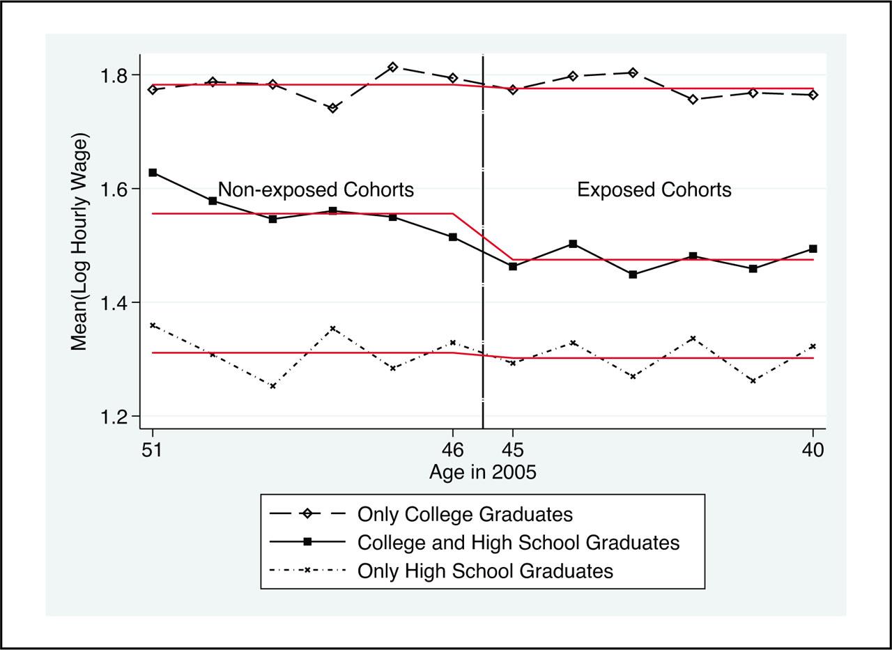
Figure 14
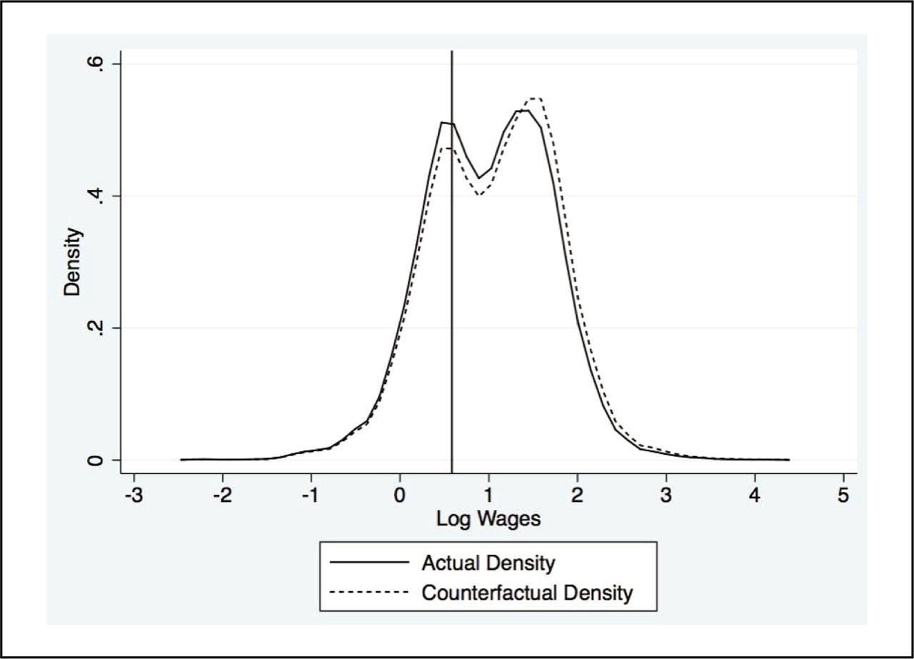
Figure 15
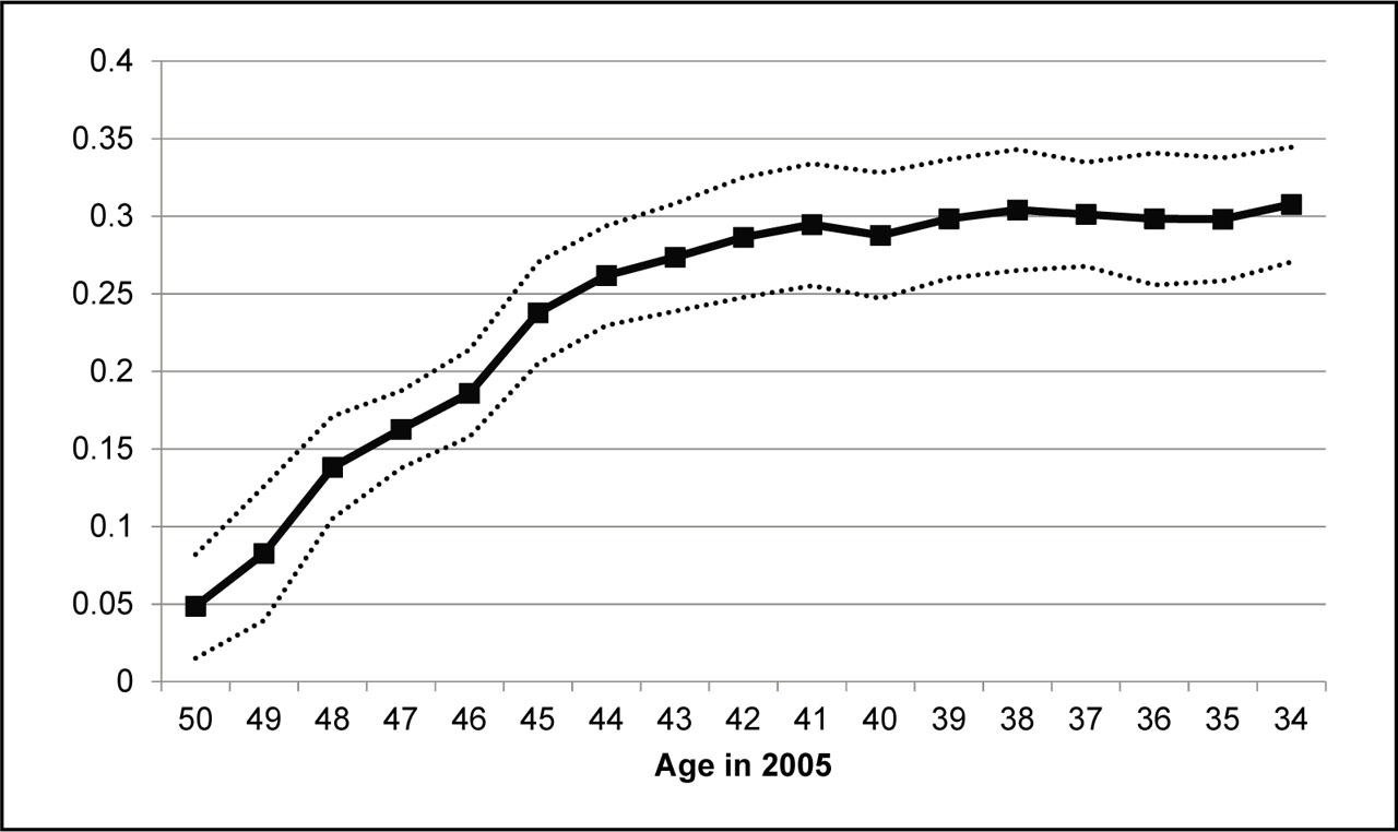
Figure 16
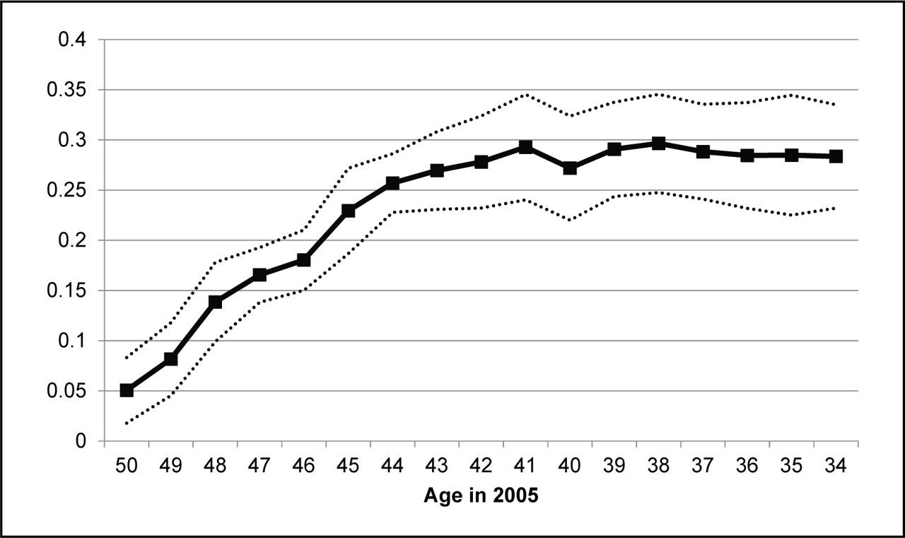
Figure 17
Fuzzy RDD estimates of the returns to college
| Dependent variable: Log hourly wage | |||
|---|---|---|---|
| [1] | [2] | [3] | |
| Treatment | 0.5716*** (0.0935) | 0.5629** (0.2425) | 0.6492* (0.3777) |
| F-statistic (discontinuity) | 140.13 | 18.63 | 8.24 |
| Region of residence | Yes | Yes | Yes |
| Urban/rural status | Yes | Yes | Yes |
| # of observations | 6,309 | 6,309 | 6,309 |
| Polynomial degree | – | linear | quadratic |
OLS and 2SLS estimates of the returns to college with adjusted missing wages
| Dependent variable: Log hourly wage | ||
|---|---|---|
| With missing values | Adjusted for missing values | |
| OLS | 0.5025*** (0.0311) | 0.5037*** (0.0310) |
| 2SLS | 0.5716*** (0.0935) | 0.5744*** (0.0935) |
| F-statistic (first stage) | 140.13 | 139.44 |
| 2SLS | 0.5588*** (0.0841) | 0.5601*** (0.0837) |
| LIML | 0.5605*** (0.0865) | 0.5618*** (0.0861) |
| F-statistic (first stage) | 25.15 | 25.04 |
| p-value Hansen's test | 0.80 | 0.80 |
| Region of residence | Yes | Yes |
| Urban/rural status | Yes | Yes |
| # of observations | 6,309 | 6,309 |
The effect of the turmoil on the probability of completing post-secondary education
| Dependent variable: Post-secondary degree==1; Otherwise==0 | ||||||
|---|---|---|---|---|---|---|
| Total | Men | Women | ||||
| [1] | [2] | [1] | [2] | [1] | [2] | |
| Age 40–45 | −0.0587*** (0.0075) | −0.0084** (0.0034) | −0.0664*** (0.0114) | −0.0102 (0.0065) | −0.0147 (0.0247) | −0.0031 (0.0053) |
| # of obs. | 18,730 | 18,852 | 15,827 | 12,798 | 2,903 | 6,054 |
| R2 | 0.0476 | 0.0570 | 0.0298 | 0.0474 | 0.0780 | 0.1077 |
Difference in the probability of graduation between the 40–45 and 46–51 age groups
| Dependent variable | |||
|---|---|---|---|
| Post-secondary | High school | Primary/Elementary | |
| Degree==1 | Degree==1 | Degree==1 | |
| Otherwise==0 | Otherwise==0 | Otherwise==0 | |
| [1] | [2] | [3] | |
| Age 40–45 | −0.0148*** (0.0051) | 0.0450*** (0.0027) | 0.0325*** (0.0092) |
| # of obs. | 74,903 | 74,903 | 74,903 |
| R2 | 0.0364 | 0.0375 | 0.0524 |
Descriptive statistics for individuals of age 34–51
| Variables | Mean |
|---|---|
| Primary or elementary sch. grad. rate | 0.63 |
| High sch. grad. rate | 0.14 |
| Post-secondary sch. grad. rate | 0.08 |
| Years of schooling | 6.36 |
| Labor force participation | 0.58 |
| Employment rate | 0.54 |
| Sample size | 115,410 |
OLS and 2SLS estimates of the returns to college with different samples
| Dependent variable: Log hourly wage | ||||
|---|---|---|---|---|
| 40–45 | 41–45 | 42–45 | 43–45 | |
| 46–51 | 47–51 | 47–50 | 47–49 | |
| [1] | [2] | [3] | [4] | |
| OLS | 0.5025*** (0.0311) | 0.5145*** (0.0333) | 0.5152*** (0.0367) | 0.5105*** (0.0342) |
| 2SLS | 0.5716*** (0.0935) | 0.5148*** (0.0690) | 0.4698*** (0.0802) | 0.4855*** (0.1016) |
| F-statistic (first stage) | 140.13 | 181.59 | 144.01 | 94.10 |
| 2SLS | 0.5588*** (0.0841) | 0.5078*** (0.0716) | 0.4774*** (0.0827) | 0.5039*** (0.1032) |
| LIML | 0.5605*** (0.0865) | 0.5076*** (0.0731) | 0.4767*** (0.0840) | 0.5037*** (0.1053) |
| F-statistic (first stage) | 25.15 | 37.43 | 36.65 | 31.97 |
| p-value Hansen's test | 0.80 | 0.72 | 0.71 | 0.61 |
| Region of residence | Yes | Yes | Yes | Yes |
| Urban/rural status | Yes | Yes | Yes | Yes |
| # of observations | 6,309 | 5,042 | 4,093 | 3,088 |
Classification of occupations and their percentages in age groups
| ISCO-88 codes | Classification | Percentage in age group | ||
|---|---|---|---|---|
| 34–39 | 40–45 | 46–51 | ||
| 12, 21, 22, 23, 24 | Corp. managers and professionals (1.53<log wage<2.07) | 13.73 | 12.00 | 18.68 |
| 31, 32, 33, 34, 41, 42 | Technicians, assoc. professionals & clerks (1.29<log wage<1.45) | 15.12 | 17.39 | 16.66 |
| 11, 13, 51, 72, 81 | Average wage earners (0.92<log wage<1.10) | 20.32 | 20.72 | 18.40 |
| 71, 73, 82, 83, 91 | Between min. wage & av. wage (0.69<log wage<0.87) | 33.29 | 34.37 | 31.28 |
| 52, 61, 62, 74, 92, 93 | Approx. less than min. wage (log wage<0.61) | 17.54 | 15.52 | 14.98 |
OLS and 2SLS estimates of the returns to college
| Dependent variable: Log hourly wage | |||
|---|---|---|---|
| [1] | [2] | [3] | |
| OLS | 0.5022*** (0.0320) | 0.5062*** (0.0304) | 0.5025*** (0.0311) |
| 2SLS | 0.5795*** (0.0965) | 0.5790*** (0.0935) | 0.5716*** (0.0935) |
| F-statistic (first stage) | 139.54 | 142.56 | 140.13 |
| 2SLS | 0.5688*** (0.0887) | 0.5659*** (0.0855) | 0.5588*** (0.0841) |
| LIML | 0.5704*** (0.0908) | 0.5676*** (0.0880) | 0.5605*** (0.0865) |
| F-statistic (first stage) | 25.01 | 25.51 | 25.15 |
| p-value Hansen's test | 0.87 | 0.80 | 0.80 |
| Region of residence | No | Yes | Yes |
| Urban/rural status | No | No | Yes |
| # of observations | 6,309 | 6,309 | 6,309 |
The effect of the turmoil on the probability of completing post-secondary education and wage
| Dependent variable | ||||||
|---|---|---|---|---|---|---|
| Post-secondary degree | Log hourly wage | |||||
| [1] | [2] | [3] | [4] | [5] | [6] | |
| Instrument (zi) | −0.1507*** (0.0214) | −0.1518*** (0.0211) | −0.1502*** (0.0207) | −0.0873*** (0.0160) | −0.0879*** (0.0159) | −0.0859*** (0.0154) |
| Region of residence | No | Yes | Yes | No | Yes | Yes |
| Urban/rural status | No | No | Yes | No | No | Yes |
| # of observations | 6,309 | 6,309 | 6,309 | 6,309 | 6,309 | 6,309 |
OLS and 2SLS estimates of the returns to college using more HLFS waves
| Dependent variable: Log hourly wage | ||
|---|---|---|
| 2005 | 2005–2008 | |
| OLS | 0.5025*** (0.0311) | 0.5380*** (0.0305) |
| 2SLS | 0.5716*** (0.0935) | 0.5644*** (0.0801) |
| F-statistic (first stage) | 140.13 | 301.03 |
| 2SLS | 0.5588*** (0.0841) | 0.5950*** (0.0883) |
| LIML | 0.5605*** (0.0865) | 0.5957*** (0.0895) |
| F-statistic (first stage) | 25.15 | 55.62 |
| p-value Hansen's test | 0.80 | 0.85 |
| Region of residence | Yes | Yes |
| Urban/rural status | Yes | Yes |
| # of observations | 6,309 | 21,717 |
Average hours worked in the main bob by educational attainment in the sample of wage earners in Turkey
| Educational attainment | # of observations | Mean |
|---|---|---|
| No schooling | 3,305 | 55.3 |
| Primary school (5 years) | 26,065 | 55.5 |
| Elementary school (8 years) | 11,046 | 54.9 |
| High school | 19,498 | 51.8 |
| Post-secondary degree | 13,396 | 44.1 |
Comparisons of age groups for male wage earners
| [1] | [2] | [3] | [4] | [5] | |
|---|---|---|---|---|---|
| Age 34–39 | 10,774 | 1.023 | 8.363 | 0.166 | 0.228 |
| Age 40–45 | 10,105 | 1.002 | 8.198 | 0.142 | 0.243 |
| Age 46–51 | 5,722 | 1.037 | 8.475 | 0.211 | 0.195 |