
Figure 1
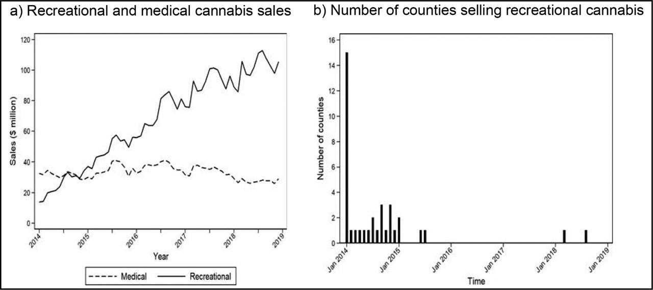
Figure 2
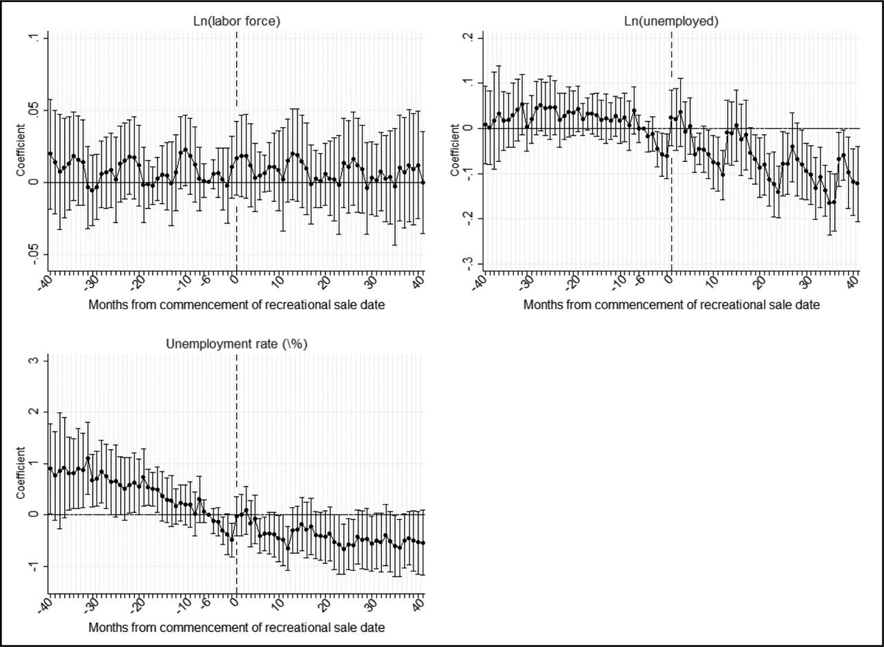
Figure 3
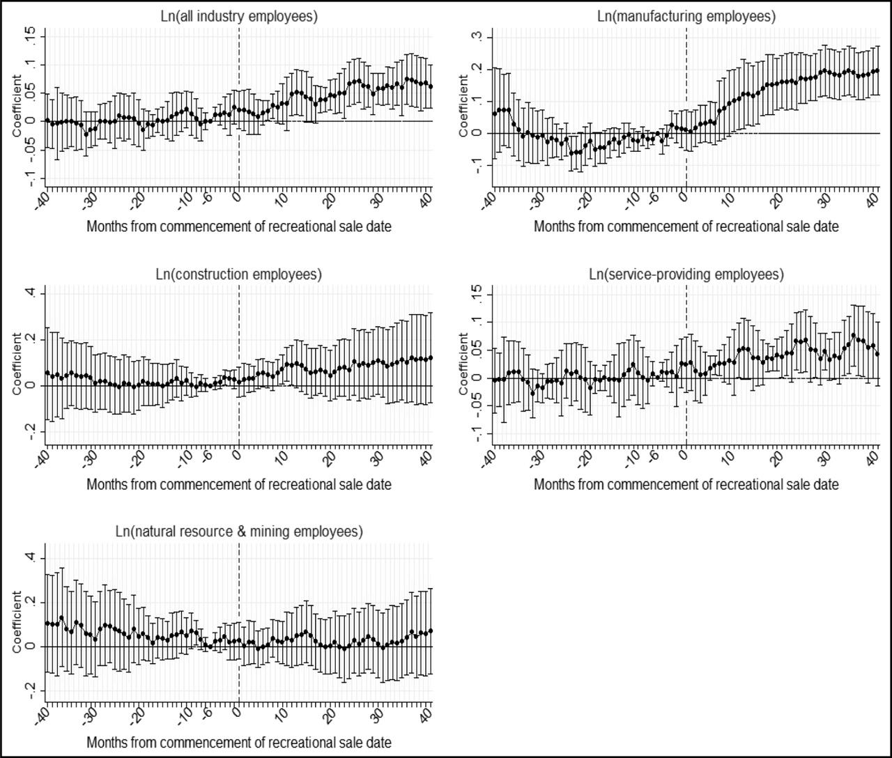
Figure 4
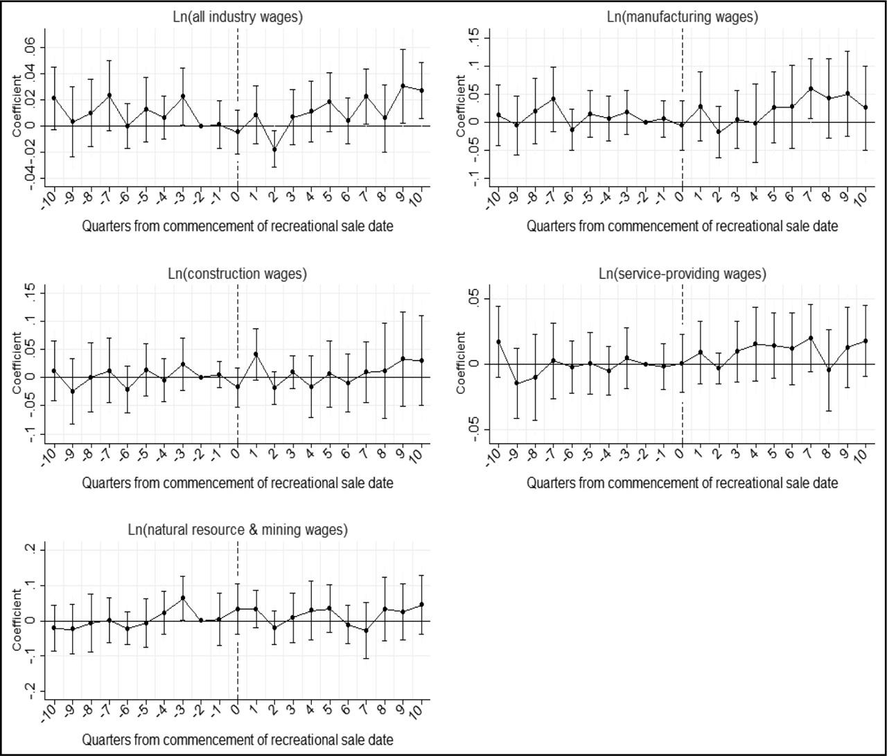
Figure 5
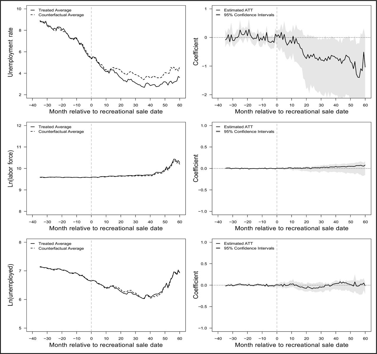
Figure 6
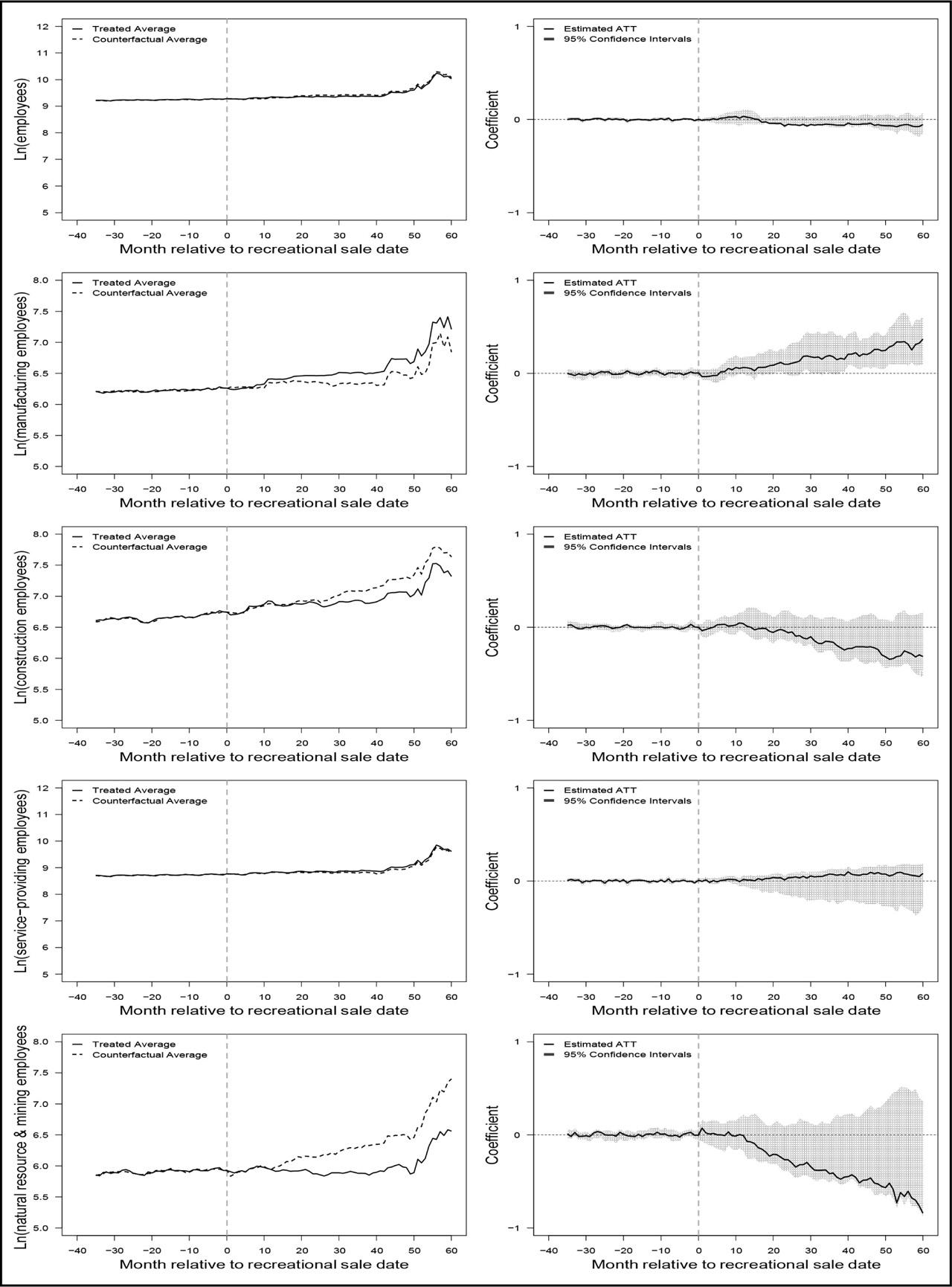
Figure 7
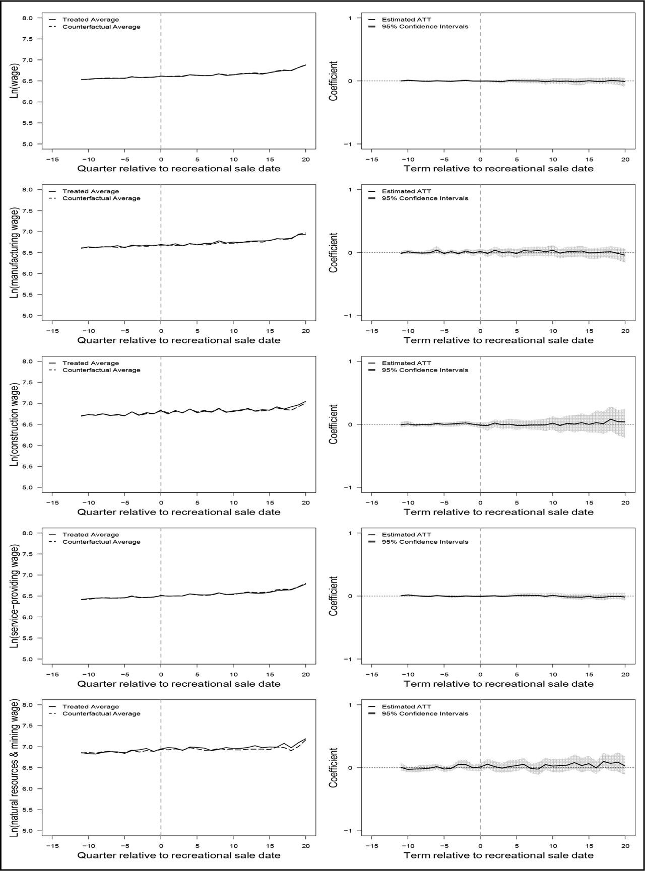
Figure A1
Figure A2
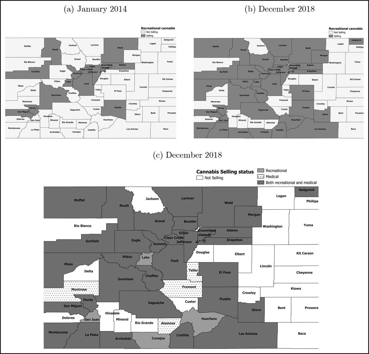
Figure A3
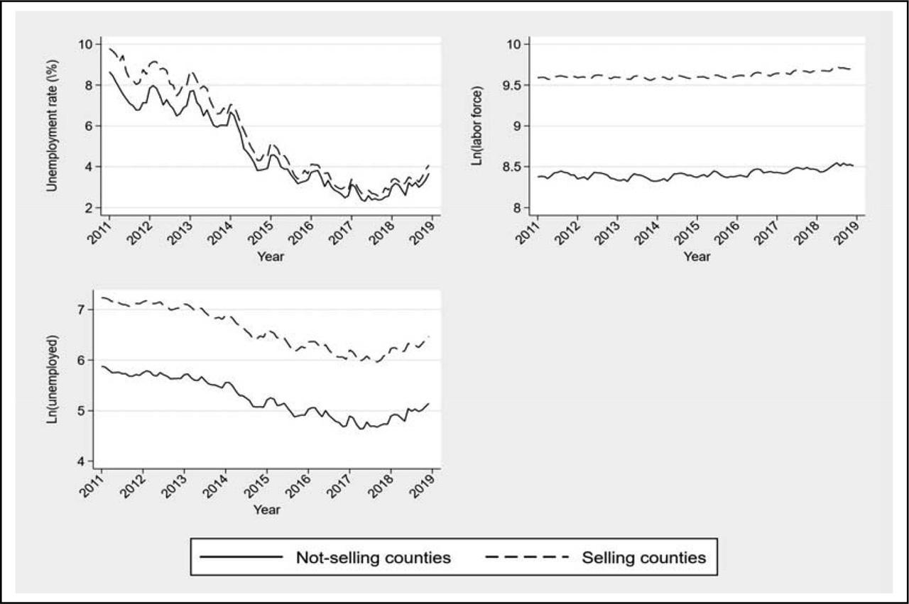
Figure A4
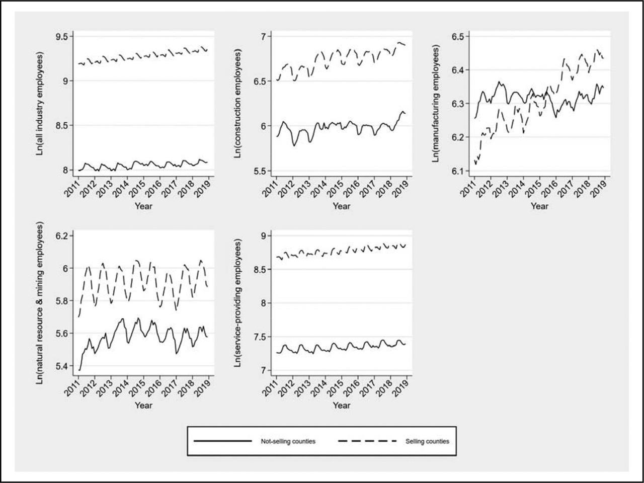
Figure A5
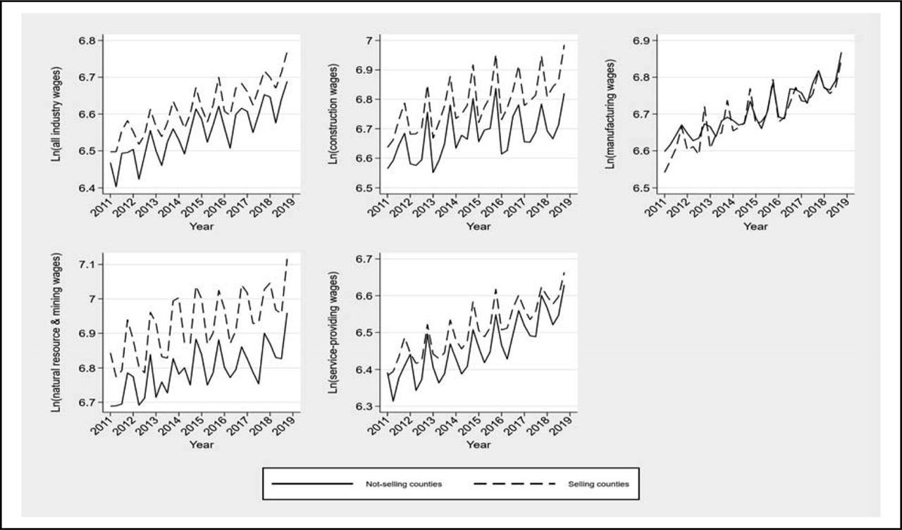
Figure A6

Figure A7
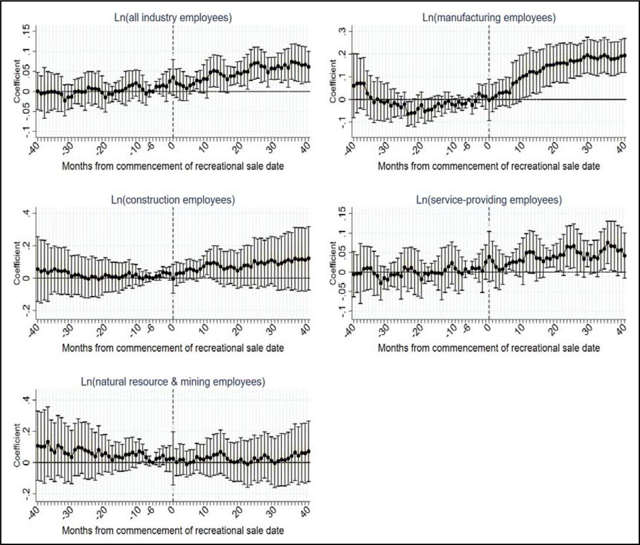
Figure A8
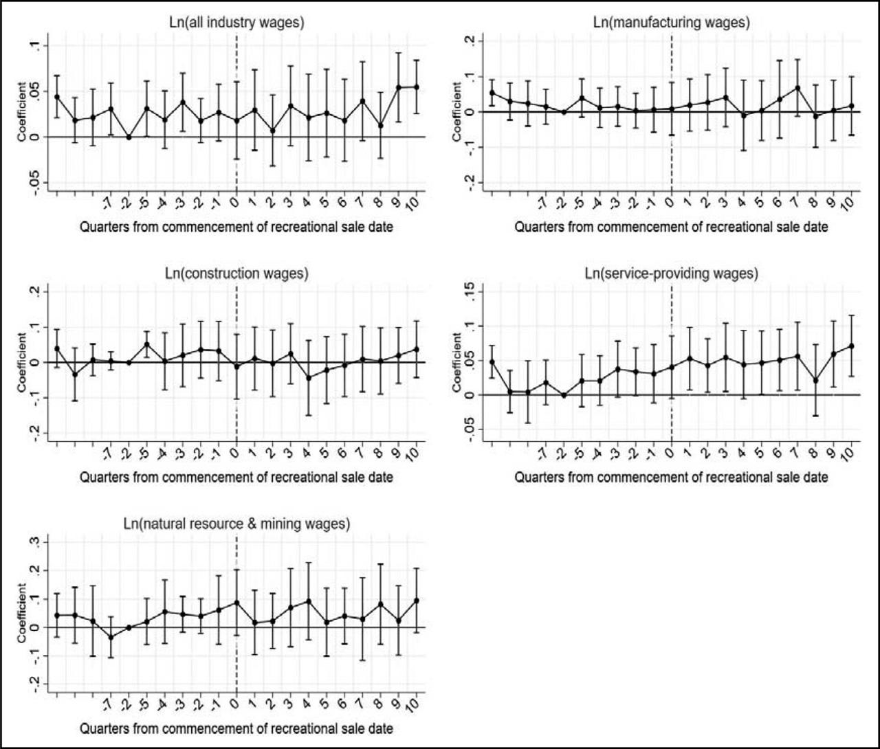
Figure A9
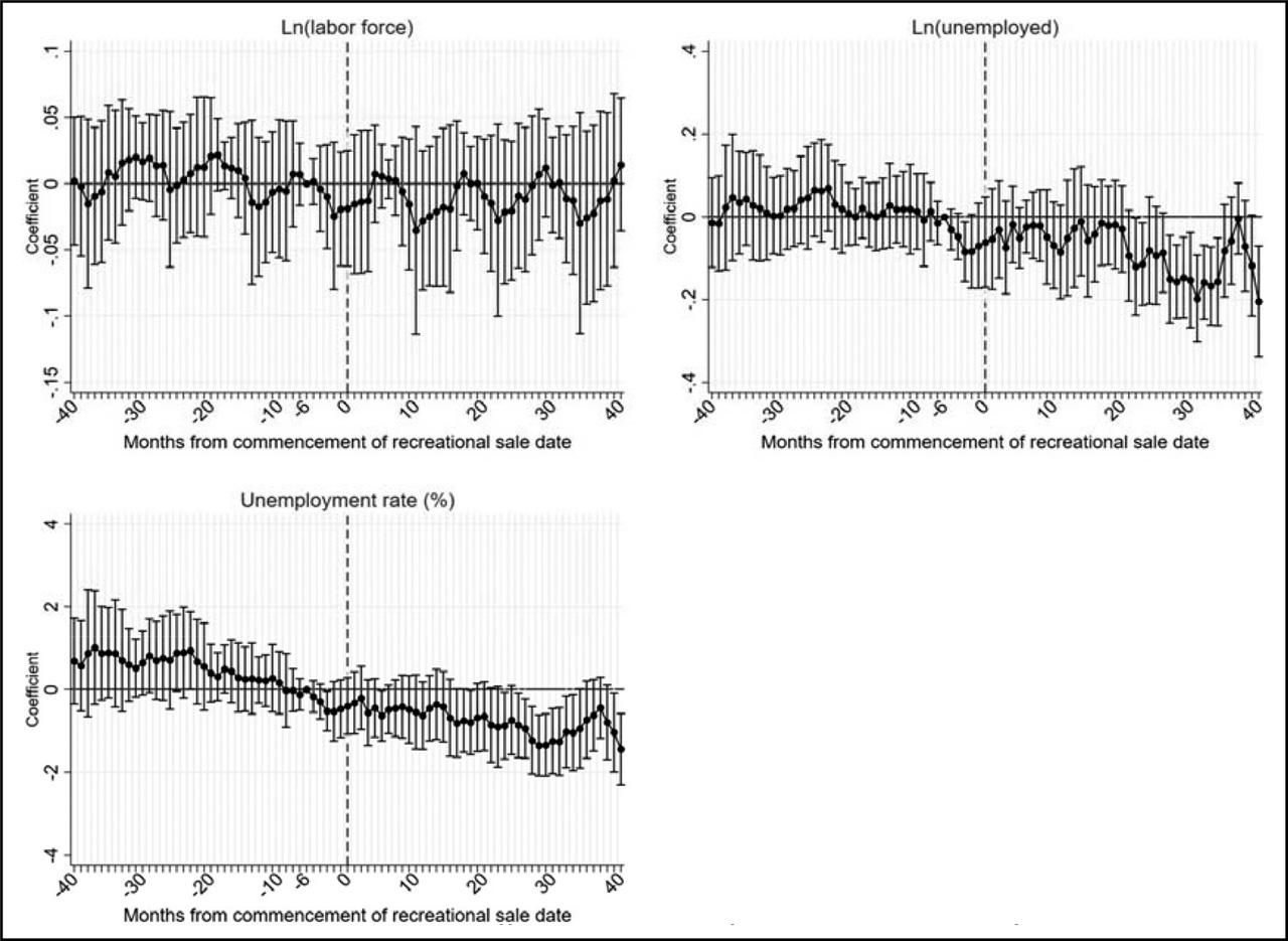
Figure A10
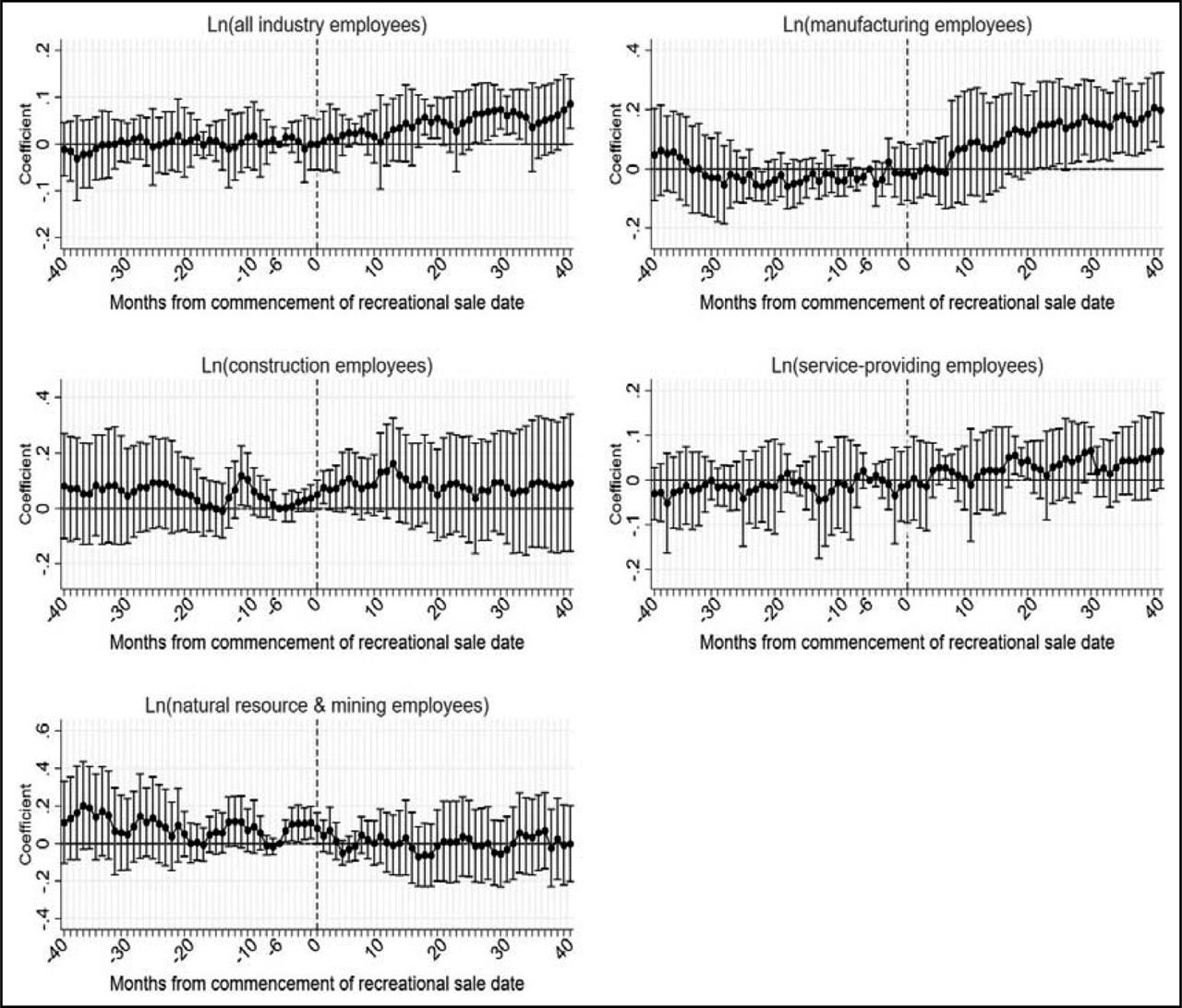
Figure A11
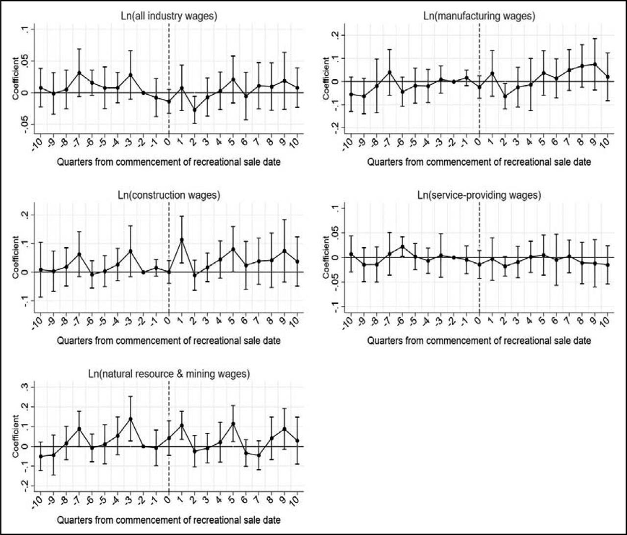
Figure A12
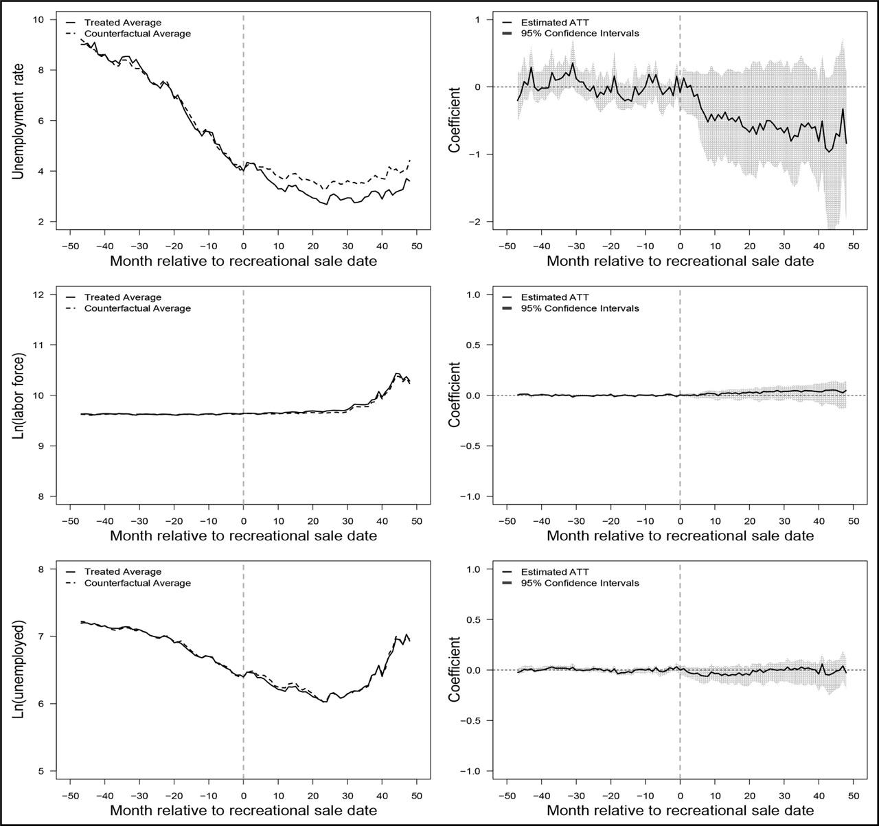
Figure A13
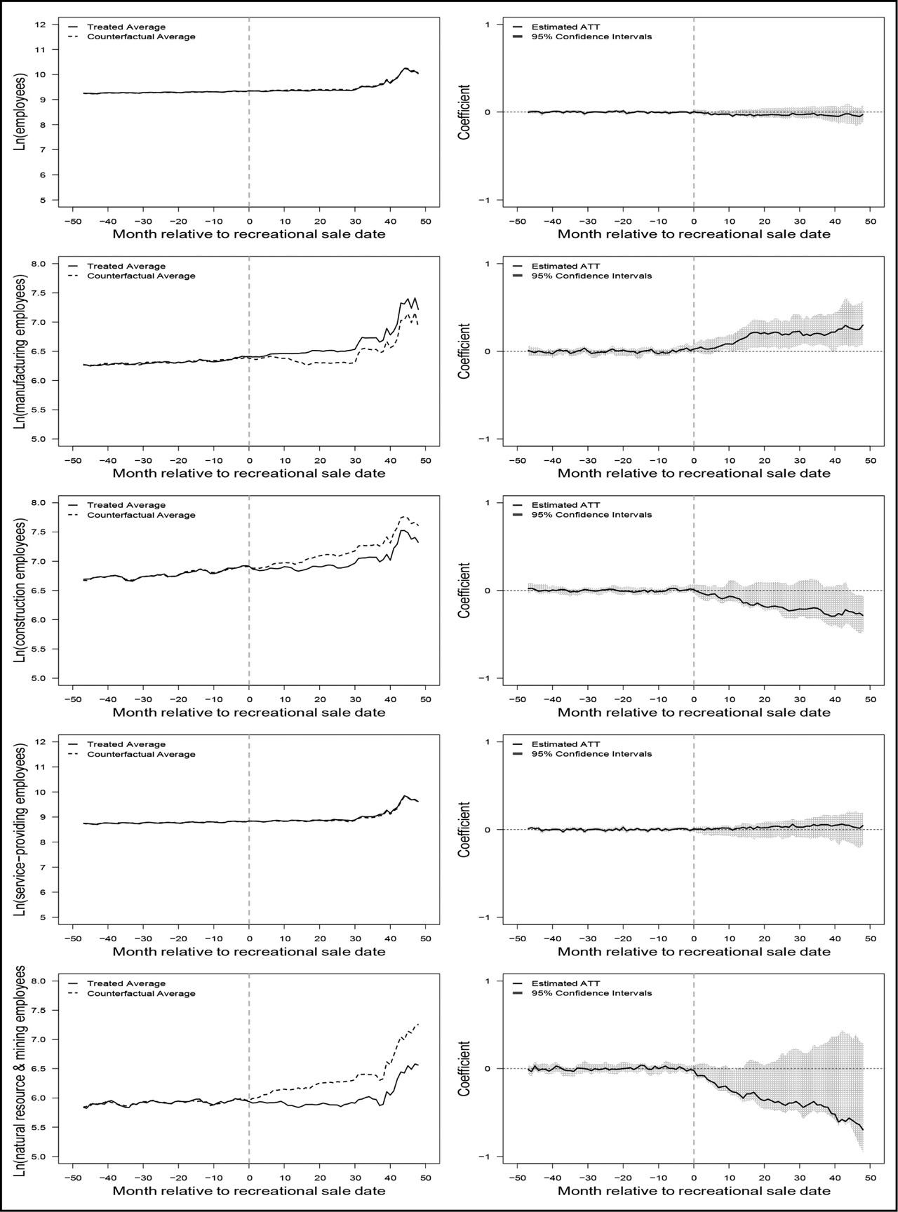
Figure A14
Descriptive statistics by treatment status
| All counties | Selling | Not selling | Differences | |||||
|---|---|---|---|---|---|---|---|---|
| Before | After | Before | After | Diff | Diff | Diff | ||
| (1) | (2) | (3) | (4) | (5) | (6) = (3)–(2) | (7) = (5)–(4) | (8) = (6)–(7) | |
| Panel A: monthly | ||||||||
| Unemployment rate, % | 5.23 | 7.86 | 3.59 | 7.09 | 3.49 | −4.268** | −3.605** | −0.663** |
| 6,144 | 1,604 | 1,948 | 972 | 1,620 | ||||
| Ln(labor force) | 9.11 | 9.48 | 9.74 | 8.38 | 8.43 | 0.258** | 0.048 | 0.21** |
| 6,144 | 1,604 | 1,948 | 972 | 1,620 | ||||
| Ln(unemployed) | 6.02 | 6.89 | 6.35 | 5.68 | 4.99 | −0.539** | −0.691** | 0.152** |
| 6,144 | 1,604 | 1,948 | 972 | 1,620 | ||||
| Ln(all industry employees) | 8.76 | 9.11 | 9.42 | 8.03 | 8.07 | 0.318** | 0.035 | 0.282** |
| 6,144 | 1,604 | 1,948 | 972 | 1,620 | ||||
| Ln(construction employees) | 6.51 | 6.50 | 6.94 | 5.94 | 6.01 | 0.436** | 0.072 | 0.364** |
| 4,608 | 1,416 | 1,752 | 540 | 900 | ||||
| Ln(manufacturing sector employees) | 6.31 | 6.06 | 6.53 | 6.32 | 6.31 | 0.470** | −0.007 | 0.477** |
| 3,936 | 1,281 | 1,503 | 432 | 720 | ||||
| Ln(natural resource and mining employees) | 5.78 | 5.86 | 5.96 | 5.55 | 5.59 | 0.105 | 0.046 | 0.059** |
| 4,608 | 1,274 | 1,510 | 684 | 1,140 | ||||
| Ln(service-providing employees) | 8.17 | 8.58 | 8.93 | 7.31 | 7.36 | 0.349** | 0.056 | 0.293** |
| 6,144 | 1,604 | 1,948 | 972 | 1,620 | ||||
| Panel B: quarterly | ||||||||
| Ln(all industry wages) | 6.59 | 6.55 | 6.67 | 6.49 | 6.59 | 0.119** | 0.097** | 0.021** |
| 2,048 | 527 | 657 | 324 | 540 | ||||
| Ln(construction wages) | 6.76 | 6.73 | 6.84 | 6.63 | 6.71 | 0.116** | 0.075* | 0.041** |
| 1,536 | 466 | 590 | 180 | 300 | ||||
| Ln(manufacturing wages) | 6.70 | 6.62 | 6.76 | 6.65 | 6.74 | 0.137** | 0.091+ | 0.046** |
| 1,312 | 421 | 507 | 144 | 240 | ||||
| Ln(natural resource and mining wages) | 6.87 | 6.86 | 6.98 | 6.74 | 6.82 | 0.119** | 0.081+ | 0.038** |
| 1,536 | 419 | 509 | 228 | 380 | ||||
| Ln(service-providing wages) | 6.49 | 6.44 | 6.57 | 6.40 | 6.50 | 0.125** | 0.098** | 0.027** |
| 2,048 | 527 | 657 | 324 | 540 | ||||
The effect of recreational dispensary entry – ATT from GSCM
| Unrate | Ln(labor force) | Ln(unemp) | |
|---|---|---|---|
| (1) | (2) | (3) | |
| Start of sales | |||
| Recreational sale | −0.566* (0.4191) | 0.024 (0.0334) | −0.006 (0.0332) |
| Ln(number of medical patients) | 0.018 (0.2547) | −0.010* (0.0084) | 0.043 (0.0713) |
| Observations | 6,144 | 6,144 | 6,144 |
The effect of recreational dispensary entry on employment – ATT from GSCM
| Ln(All) | Ln(Cons) | Ln(Manu) | Ln(NR) | Ln(Service) | |
|---|---|---|---|---|---|
| (1) | (2) | (3) | (4) | (5) | |
| Start of sales | |||||
| Recreational sale | −0.035 (0.0203) | −0.120 (0.0804) | 0.137** (0.0562) | −0.298 (0.1314) | 0.042 (0.0587) |
| Ln(number of medical patients) | 0.001 (0.0148) | −0.502 (0.2495) | 0.097 (0.1150) | −0.010 (0.0894) | 0.007 (0.0229) |
| Observations | 6,144 | 4,608 | 3,936 | 4,608 | 6,144 |
Sources for our variable of interest
| Variable type | Source | Chronology |
|---|---|---|
| Unemployed, Labor force, and Unemployment rate (2011–2018) | Local Area Unemployment Statistics (LAUS) | |
| Employees and wages (2011–2018) | Quarterly Census of Employment and Wages (QCEW) | |
| Recreational cannabis sales (2014–2018) | Colorado Department of Revenue (CDOR) | |
| Medical cannabis patients (2011–2018) | Colorado Department of Public Health and Environment (CDPHE) | |
| Population (2011–2018) | United States Census Bureau |
The effect of recreational dispensary entry and sales on employment – regression analysis
| All | Cons | Manu | NR | Service | |
|---|---|---|---|---|---|
| (1) | (2) | (3) | (4) | (5) | |
| Panel A: amount of sales | |||||
| Recreational sale | 0.054* (0.0223) | 0.065 (0.0754) | 0.094 (0.0700) | −0.007 (0.1125) | 0.035+ (0.0205) |
| Recreational sale=1 × < 70 km not-sellingmy=1 | −0.014 (0.0221) | −0.010 (0.0682) | 0.048 (0.0726) | −0.011 (0.1112) | 0.005 (0.0198) |
| Ln(number of medical patients) | −0.021 (0.0153) | −0.173+ (0.0946) | −0.195** (0.0648) | 0.173 (0.1135) | −0.027 (0.0184) |
| R2 | 0.998 | 0.989 | 0.996 | 0.970 | 0.998 |
| Observations | 6,144 | 4,608 | 3,936 | 4,608 | 6,144 |
County-level summary statistics
| Mean | SD | Min | Max | N | |
|---|---|---|---|---|---|
| Panel A: monthly | |||||
| Unemployment rate (%) | 5.23 | 2.77 | 1.1 | 17.4 | 6,144 |
| Labor force | 44,682 | 90,397 | 273 | 417,717 | 6,144 |
| Unemployed | 2,268 | 5,017 | 7 | 33,083 | 6,144 |
| All industry employees | 37,909 | 84,671 | 195 | 524,919 | 6,144 |
| Construction employees | 2,720 | 5,099 | 14 | 24,163 | 4,992 |
| Manufacturing sector employees | 2,929 | 5,427 | 10 | 21,436 | 4,512 |
| Natural resource and mining employees | 802 | 1,821 | 8 | 13,120 | 5,088 |
| Service-providing employees | 26,692 | 62,824 | 81 | 401,921 | 6,144 |
| Amount of recreational sales | 629,296 | 2,712,311 | 0 | 35,343,772 | 6,144 |
| Number of medical patients | 1,622 | 3,568 | 2 | 20,976 | 6,144 |
| Panel B: quarterly | |||||
| All industry wages | 749.06 | 200.83 | 410 | 2,102 | 2,048 |
| Construction wages | 881.75 | 227.47 | 415 | 2,489 | 1,664 |
| Manufacturing wages | 844.94 | 339.17 | 310 | 2,650 | 1,504 |
| Natural resource and mining wages | 1,071.30 | 641.53 | 376 | 6,475 | 1,696 |
| Service-providing wages | 684.91 | 216.46 | 294 | 2,619 | 2,048 |
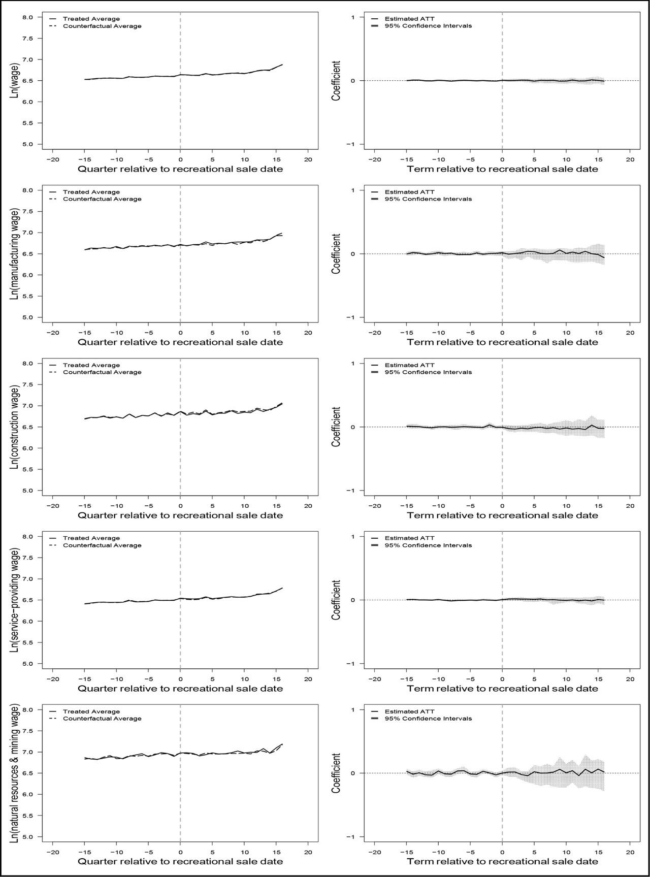
Event study estimates post-dispensary entry periods for wages, by industry
| All | Cons | Manu | NR | Service | |
|---|---|---|---|---|---|
| (1) | (2) | (3) | (4) | (5) | |
| event0:treat | −0.005 | −0.017 | −0.006 | 0.033 | 0.000 |
| event1:treat | 0.008 | 0.041+ | 0.028 | 0.033 | 0.009 |
| event2:treat | −0.018* | −0.018 | −0.018 | −0.020 | −0.003 |
| event3:treat | 0.007 | 0.010 | 0.005 | 0.008 | 0.010 |
| event4:treat | 0.011 | −0.016 | −0.002 | 0.029 | 0.015 |
| event5:treat | 0.018 | 0.007 | 0.026 | 0.034 | 0.014 |
| event6:treat | 0.004 | −0.010 | 0.027 | −0.011 | 0.012 |
| event7:treat | 0.023* | 0.010 | 0.059* | −0.027 | 0.020 |
| event8:treat | 0.006 | 0.012 | 0.042 | 0.034 | −0.005 |
| event9:treat | 0.030* | 0.033 | 0.051 | 0.025 | 0.013 |
| event10:treat | 0.027* | 0.030 | 0.026 | 0.045 | 0.017 |
| event>10:treat | 0.018 | 0.029 | 0.023 | 0.039 | −0.004 |
| Linear combination | |||||
| Coefficient | 0.011 | 0.009 | 0.022 | 0.019 | 0.008 |
| SE | 0.0076 | 0.0239 | 0.0265 | 0.0269 | 0.0093 |
| Weighted linear combination | |||||
| Coefficient | 0.013 | 0.017 | 0.022 | 0.026 | 0.004 |
| SE | 0.0092 | 0.0314 | 0.0298 | 0.0323 | 0.0105 |
| R2 | 0.938 | 0.780 | 0.933 | 0.910 | 0.925 |
| Observations | 2,048 | 1,536 | 1,312 | 1,536 | 2,048 |
Event study estimates post-dispensary entry periods
| Unrate | Ln(labor force) | Ln(unemp) | |
|---|---|---|---|
| (1) | (2) | (3) | |
| event0:treat | 0.382* | 0.041* | 0.113** |
| event1:treat | 0.320+ | 0.043* | 0.093** |
| event2:treat | 0.440 | 0.041* | 0.112* |
| event3:treat | 0.179 | 0.031+ | 0.064+ |
| event4:treat | 0.192 | −0.007 | 0.025 |
| event5:treat | −0.224 | −0.003 | −0.062** |
| event6:treat | −0.283+ | 0.001 | −0.060** |
| event7:treat | −0.300 | 0.009 | −0.066* |
| event8:treat | −0.373 | 0.013 | −0.087** |
| event9:treat | −0.486* | 0.015 | −0.103** |
| event10:treat | −0.393 | 0.016 | −0.085* |
| event11:treat | −0.564* | 0.036* | −0.105** |
| event12:treat | −0.026 | 0.040+ | 0.042 |
| event13:treat | −0.119 | 0.038+ | 0.012 |
| event14:treat | 0.133 | 0.030 | 0.039 |
| event15:treat | 0.058 | 0.023 | 0.014 |
| event16:treat | 0.227 | −0.014 | 0.010 |
| event17:treat | −0.092 | −0.014 | −0.081* |
| event18:treat | −0.126 | −0.011 | −0.099** |
| event19:treat | −0.246 | −0.004 | −0.137** |
| event20:treat | −0.163 | −0.004 | −0.117** |
| event21:treat | −0.302 | −0.003 | −0.132** |
| event22:treat | −0.266 | −0.002 | −0.119** |
| event23:treat | −0.411 | 0.024 | −0.140** |
| event24:treat | −0.263 | 0.021 | −0.030 |
| event25:treat | −0.249 | 0.023 | −0.028 |
| event26:treat | 0.098 | 0.019 | 0.036 |
| event27:treat | 0.143 | 0.008 | 0.029 |
| event28:treat | 0.195 | −0.026 | −0.000 |
| event29:treat | 0.051 | −0.017 | −0.035 |
| event30:treat | 0.040 | −0.010 | −0.046 |
| event31:treat | −0.024 | −0.002 | −0.069+ |
| event32:treat | 0.050 | −0.003 | −0.058 |
| event33:treat | −0.191 | −0.003 | −0.109** |
| event34:treat | −0.341 | −0.003 | −0.157** |
| event35:treat | −0.524+ | 0.021 | −0.200** |
| event36:treat | −0.412 | 0.015 | −0.048 |
| event37:treat | −0.499+ | 0.019 | −0.079** |
| event38:treat | −0.309 | 0.015 | −0.091 |
| event39:treat | −0.266 | 0.011 | −0.096* |
| event40:treat | −0.023 | −0.024 | −0.052 |
| event>40:treat | 0.037 | −0.002 | −0.020 |
| Linear combination | |||
| Combo coefficient | −0.117 | 0.010 | −0.046* |
| Combo SE | 0.2257 | 0.0139 | 0.0212 |
| Weighted linear combination | |||
| Combo coefficient | −0.073 | 0.006 | −0.038+ |
| Combo SE | 0.2433 | 0.0148 | 0.0218 |
| R2 | 0.880 | 0.999 | 0.996 |
| Observations | 4,512 | 4,512 | 4,512 |
The effect of recreational dispensary entry and sales on the unemployment rate, Ln(labor force), and Ln(unemployed) – regression analysis
| Unrate | Ln(labor force) | Ln(unemp) | |
|---|---|---|---|
| (1) | (2) | (3) | |
| Panel A: start of sales | |||
| Recreational sale | −0.718** (0.2428) | −0.014 (0.0105) | −0.078** (0.0200) |
| Ln(number of medical patients) | −0.607* (0.2714) | 0.001 (0.0111) | −0.021 (0.0250) |
| Ln(population) | 1.158 (2.4361) | 0.531** (0.1261) | 0.338+ (0.1900) |
| R2 | 0.882 | 0.999 | 0.995 |
| Observations | 6,144 | 6,144 | 6,144 |
| Panel B: amount of sales | |||
| $0 < sales ≤$500,000 (0.2720) | −0.752** (0.0099) | −0.009 (0.0224) | −0.066** |
| Sales >$500,000 (0.2515) | −0.669** (0.0125) | −0.021 (0.0251) | −0.094** |
| Ln(number of medical patients) | −0.601** (0.2737) | 0.000 (0.0108) | −0.023 (0.0260) |
| Ln(population) | 1.069 (2.4483) | 0.543** (0.1276) | 0.369+ (0.1872) |
| R2 | 0.882 | 0.999 | 0.995 |
| Observations | 6,144 | 6,144 | 6,144 |
Event study estimates post-dispensary entry periods for employees, by industry
| All | Cons | Manu | NR | Service | |
|---|---|---|---|---|---|
| (1) | (2) | (3) | (4) | (5) | |
| event0:treat | 0.020 | 0.017 | 0.010 | 0.028 | 0.024 |
| event1:treat | 0.020 | 0.027 | 0.006 | 0.003 | 0.028 |
| event2:treat | 0.017 | 0.033 | 0.016 | 0.020 | 0.013 |
| event3:treat | 0.013 | 0.032 | 0.029 | 0.020 | 0.006 |
| event4:treat | 0.008 | 0.052+ | 0.030 | −0.010 | 0.008 |
| event5:treat | 0.015 | 0.058+ | 0.036 | 0.001 | 0.018 |
| event6:treat | 0.019* | 0.050+ | 0.030 | 0.006 | 0.023** |
| event7:treat | 0.028* | 0.042 | 0.070 | 0.037 | 0.027* |
| event8:treat | 0.025+ | 0.057* | 0.077 | 0.025 | 0.026 |
| event9:treat | 0.031+ | 0.073* | 0.093+ | 0.020 | 0.031 |
| event10:treat | 0.031 | 0.093* | 0.103* | 0.036 | 0.028 |
| event11:treat | 0.048* | 0.090* | 0.108* | 0.030 | 0.050* |
| event12:treat | 0.052* | 0.096+ | 0.123* | 0.049 | 0.052+ |
| event13:treat | 0.051* | 0.088 | 0.123* | 0.053 | 0.051+ |
| event14:treat | 0.044+ | 0.072 | 0.117* | 0.069 | 0.036 |
| event15:treat | 0.039+ | 0.056 | 0.126* | 0.051 | 0.036 |
| event16:treat | 0.030+ | 0.063 | 0.140** | 0.025 | 0.028 |
| event17:treat | 0.039** | 0.071 | 0.152** | 0.008 | 0.037** |
| event18:treat | 0.039** | 0.063 | 0.152** | 0.002 | 0.035** |
| event19:treat | 0.047** | 0.046 | 0.154** | 0.006 | 0.041** |
| event20:treat | 0.044** | 0.060 | 0.160** | 0.020 | 0.038* |
| event21:treat | 0.050** | 0.079 | 0.161** | 0.001 | 0.045* |
| event22:treat | 0.049* | 0.080 | 0.163** | −0.010 | 0.045+ |
| event23:treat | 0.066** | 0.070 | 0.158** | 0.002 | 0.066* |
| event24:treat | 0.070** | 0.106 | 0.173** | 0.029 | 0.064* |
| event25:treat | 0.072** | 0.090 | 0.169** | 0.013 | 0.067* |
| event26:treat | 0.063** | 0.098 | 0.172** | 0.029 | 0.051+ |
| event27:treat | 0.062** | 0.089 | 0.175** | 0.048 | 0.050* |
| event28:treat | 0.048* | 0.101 | 0.188** | 0.034 | 0.034 |
| event29:treat | 0.057** | 0.112 | 0.197** | 0.012 | 0.047** |
| event30:treat | 0.057** | 0.102 | 0.188** | −0.003 | 0.033+ |
| event31:treat | 0.063** | 0.085 | 0.185** | 0.009 | 0.040+ |
| event32:treat | 0.059** | 0.093 | 0.180** | 0.019 | 0.036 |
| event33:treat | 0.067** | 0.103 | 0.189** | 0.017 | 0.054* |
| event34:treat | 0.059* | 0.114 | 0.197** | 0.027 | 0.060* |
| event35:treat | 0.074** | 0.103 | 0.189** | 0.042 | 0.077** |
| event36:treat | 0.073** | 0.122 | 0.179** | 0.065 | 0.067* |
| event37:treat | 0.070** | 0.115 | 0.180** | 0.044 | 0.067* |
| event38:treat | 0.066** | 0.117 | 0.184** | 0.062 | 0.055+ |
| event39:treat | 0.067** | 0.113 | 0.193** | 0.060 | 0.057+ |
| event40:treat | 0.062** | 0.123 | 0.195** | 0.071 | 0.043 |
| event>40:treat | 0.076** | 0.107 | 0.171** | 0.105 | 0.054+ |
| Linear combination | |||||
| Coefficient | 0.047* | 0.080 | 0.134** | 0.028 | 0.042* |
| SE | 0.0145 | 0.0542 | 0.0333 | 0.0563 | 0.0188 |
| Weighted linear combination | |||||
| Coefficient | 0.054** | 0.086 | 0.142** | 0.046 | 0.044* |
| SE | 0.0154 | 0.0657 | 0.0328 | 0.0642 | 0.0204 |
| R2 | 0.998 | 0.989 | 0.996 | 0.970 | 0.998 |
| Observations | 6,144 | 4,608 | 3,936 | 4,608 | 6,144 |
Effect of preexisting county-level economic conditions on dispensary entry
| Dependent variable=Rcmy | 6-month change | 1-year change |
|---|---|---|
| Pop change | 0.000* (0.0000) | 0.000 (0.0000) |
| Unrate change | 0.013* (0.0050) | 0.039* (0.0191) |
| Ln(labor force change) | −0.049 (0.0497) | −0.379 (0.3405) |
| Ln(Unemp change) | 0.021 (0.0256) | −0.005 (0.0554) |
| Ln(All Emp change) | 0.007 (0.0345) | −0.032 (0.1537) |
| Ln(Cons Emp change) | 0.022 (0.0478) | 0.026 (0.0593) |
| Ln(Manu Emp change) | 0.097 (0.0839) | 0.149 (0.0926) |
| Ln(NR Emp change) | 0.028 (0.0381) | 0.030 (0.0874) |
| Ln(Service Emp change) | −0.002 (0.0186) | −0.122 (0.1650) |
| Ln(All wage change) | 0.053 (0.0549) | 0.084 (0.1125) |
| Ln(Cons wage change) | 0.022 (0.0473) | 0.019 (0.080) |
| Ln(Manu wage change) | −0.009 (0.0407) | −0.028 (0.0875) |
| Ln(NR wage change) | −0.011 (0.019) | −0.100 (0.0697) |
| Ln(Service wage change) | −0.024 (0.0310) | −0.001 (0.1016) |
Multiple inference – adjusted p–value
| Dependent variable | p–value | Sharpened q–values |
|---|---|---|
| Panel A: monthly | ||
| Unemployment rate | 0.009** | 0.024* |
| Ln(labor force) | 0.915 | 1 |
| Ln(unemployed) | 0.001** | 0.007** |
| Ln(all industry employees) | 0.005** | 0.019* |
| Ln(construction employees) | 0.292 | 0.638 |
| Ln(manufacturing sector employees) | 0.001** | 0.007** |
| Ln(natural resource and mining employees) | 0.823 | 1 |
| Ln(service–providing employees) | 0.015* | 0.031* |
| Panel B: quarterly | ||
| Ln(All industry wages) | 0.952 | 1 |
| Ln(Construction wages) | 0.761 | 1 |
| Ln(Manufacturing wages) | 0.594 | 1 |
| Ln(Natural resource and mining wages) | 0.424 | 0.941 |
| Ln(Service–providing wages) | 0.74 | 1 |
Effect of recreational dispensary entry and sales on the unemployment rate (Unrate), Ln(labor force), and Ln(unemployed) – regression analysis
| Unrate | Ln(labor force) | Ln(unemp) | |
|---|---|---|---|
| (1) | (2) | (3) | |
| Panel A: start of sales | |||
| Recreational sale | −0.684** (0.2522) | 0.001 (0.0115) | −0.068** (0.0194) |
| Ln(number of medical patients) | −0.621* (0.2692) | −0.006 (0.0126) | −0.025 (0.0249) |
| Linear combination | |||
| Coefficient | −0.407* | 0.008 | −0.068** |
| SE | (0.2264) | (0.0125) | (0.0238) |
| Weighted linear combination | |||
| Coefficient | −0.339 | 0.008 | −0.060* |
| SE | (0.2433) | (0.0133) | (0.0243) |
| R2 | 0.881 | 0.999 | |
| Observations | 6,144 | 6,144 | 6,144 |
| Panel B: amount of sales | |||
| $0 < sales ≤ $500,000 | −0.727** (0.2803) | 0.003 (0.0109) | −0.058** (0.0223) |
| Sales > $500,000 | −0.630** (0.2641) | −0.001 (0.0144) | −0.081** (0.0245) |
| Ln(number of medical patients) | −0.613** (0.2724) | −0.006 (0.0128) | −0.027 (0.0261) |
| R2 | 0.882 | 0.999 | 0.995 |
| Observations | 6,144 | 6,144 | 6,144 |
The effect of recreational dispensary entry on the unemployment rate (Unrate), Ln(labor force), and Ln(unemployed) – regression analysis
| Unrate | Ln(labor force) | Ln(unemp) | |
|---|---|---|---|
| (1) | (2) | (3) | |
| Panel A: start of sales | |||
| Recreational sale | −0.688** (0.2548) | 0.000 (0.0116) | −0.069** (0.0197) |
| Ln(number of medical patients) | −0.618* (0.2703) | −0.006 (0.0127) | −0.025 (0.0250) |
| R2 | 0.881 | 0.999 | 0.995 |
| Observations | 6,048 | 6,048 | 6,048 |
| Panel B: amount of sales | |||
| $0 < sales ≤ $500,000 | −0.729** (0.2809) | 0.003 (0.0109) | −0.058** (0.0223) |
| Sales > $500,000 | −0.634** (0.2693) | −0.003 (0.0146) | −0.083** (0.0253) |
| Ln(number of medical patients) | −0.610** (0.2736) | −0.006 (0.0128) | −0.027 (0.0263) |
| R2 | 0.881 | 0.999 | 0.995 |
| Observations | 6,048 | 6,048 | 6,048 |
The effect of recreational dispensary entry on employment – regression analysis
| All | Cons | Manu | NR | Service | |
|---|---|---|---|---|---|
| (1) | (2) | (3) | (4) | (5) | |
| Panel A: start of sales | |||||
| Recreational sale | 0.043** (0.0152) | 0.054 (0.0552) | 0.131** (0.0360) | −0.019 (0.0674) | 0.037* (0.0155) |
| Ln(number of medical patients) | −0.022 (0.0143) | −0.175+ (0.0918) | −0.190** (0.0606) | 0.170 (0.1178) | −0.026 (0.0183) |
| R2 | 0.998 | 0.988 | 0.995 | 0.965 | 0.998 |
| Observations | 6,048 | 4,512 | 3,840 | 4,512 | 6,048 |
| Panel B: amount of sales | |||||
| $0 < sales ≤ $500,000 | 0.029+ (0.0155) | 0.053 (0.0489) | 0.148** (0.0381) | −0.032 (0.0661) | 0.025 (0.0173) |
| Sales > $500,000 | 0.062** (0.0181) | 0.055 (0.0677) | 0.110** (0.0387) | −0.003 (0.0829) | 0.054** (0.0172) |
| Ln(number of medical patients) | −0.019 (0.0149) | −0.175+ (0.0921) | −0.195** (0.0593) | 0.173 (0.1182) | −0.024 (0.0181) |
| R2 | 0.998 | 0.988 | 0.995 | 0.965 | 0.998 |
| Observations | 6,048 | 4,512 | 3,840 | 4,512 | 6,048 |
The effect of recreational dispensary entry and sales on the unemployment rate (Unrate), Ln(labor force), and Ln(unemployed) – regression analysis
| Unrate | Ln(labor force) | Ln(unemp) | |
|---|---|---|---|
| (1) | (2) | (3) | |
| Panel A: amount of sales | |||
| Recreational sale | −0.365 (0.3154) | −0.004 (0.0195) | −0.089** (0.0299) |
| Recreational sale=1 × < 70km not-sellingmy=1 | −0.430 (0.2864) | 0.006 (0.0183) | 0.028 (0.0311) |
| Ln(number of medical patients) | −0.580* (0.2774) | −0.006 (0.0132) | −0.028 (0.0258) |
| R2 | 0.882 | 0.999 | 0.995 |
| Observations | 6,144 | 6,144 | 6,144 |
The effect of recreational dispensary entry on wage – ATT from GSCM
| Ln(All) | Ln(Cons) | Ln(Manu) | Ln(NR) | Ln(Service) | |
|---|---|---|---|---|---|
| (1) | (2) | (3) | (4) | (5) | |
| Start of sales | |||||
| Recreational sale | −0.003 (0.0178) | 0.007 (0.0531) | 0.011 (0.0321) | 0.036 (0.0424) | −0.004 (0.0152) |
| Ln(number of medical patients) | −0.017 (0.0161) | 0.006 (0.1258) | −0.027 (0.0474) | 0.114** (0.0698) | −0.010 (0.0438) |
| Observations | 6144 | 4608 | 3936 | 4608 | 6144 |
The effect of recreational dispensary entry and sales on wages – regression analysis
| All | Cons | Manu | NR | Service | |
|---|---|---|---|---|---|
| (1) | (2) | (3) | (4) | (5) | |
| Panel A: amount of sales | |||||
| Recreational sale | 0.003 (0.0148) | 0.036 (0.0288) | 0.007 (0.0214) | 0.043 (0.0368) | 0.006 (0.0135) |
| Recreational sale=1 × < 70 km not-sellingmy=1 | −0.004 (0.0135) | −0.039 (0.0250) | 0.004 (0.0341) | −0.024 (0.0258) | −0.003 (0.0112) |
| Ln(number of medical patients) | 0.004 (0.0113) | −0.077 (0.0476) | −0.036 (0.0306) | 0.067+ (0.0345) | 0.002 (0.0178) |
| R2 | 0.937 | 0.778 | 0.932 | 0.909 | 0.925 |
| Observations | 2,048 | 1,536 | 1,312 | 1,536 | 2,048 |
The effect of recreational dispensary entry on wages – regression analysis
| All | Cons | Manu | NR | Service | |
|---|---|---|---|---|---|
| (1) | (2) | (3) | (4) | (5) | |
| Panel A: start of sales | |||||
| Recreational sale | 0.001 (0.0101) | 0.007 (0.0265) | 0.010 (0.0197) | 0.028 (0.0318) | 0.004 (0.0127) |
| Ln(number of medical patients) | 0.004 (0.0113) | −0.081+ (0.0469) | −0.036 (0.0271) | 0.061+ (0.0341) | 0.002 (0.0176) |
| R2 | 0.932 | 0.768 | 0.932 | 0.900 | 0.919 |
| Observations | 2,016 | 1,504 | 1,280 | 1,504 | 2,016 |
| Panel B: amount of sales | |||||
| $0 < sales ≤ $500,000 | 0.006 (0.0106) | 0.008 (0.0254) | 0.025 (0.0249) | 0.029 (0.0294) | 0.009 (0.0139) |
| Sales > $500,000 | −0.007 (0.0119) | 0.006 (0.0338) | −0.012 (0.0196) | 0.026 (0.0384) | −0.004 (0.0134) |
| Ln(number of medical patients) | 0.002 (0.0109) | −0.081+ (0.0469) | −0.041 (0.0280) | 0.061+ (0.0339) | 0.001 (0.0173) |
| R2 | 0.932 | 0.768 | 0.932 | 0.900 | 0.919 |
| Observations | 2,016 | 1,504 | 1,280 | 1,504 | 2,016 |
The effect of recreational dispensary entry and sales on the Unemployment Rate (Unrate), Ln(labor force), and Ln(unemployed) – regression analysis
| Unrate | Ln(labor force) | Ln(unemp) | |
|---|---|---|---|
| (1) | (2) | (3) | |
| Panel A: amount of sales | |||
| Recreational sale | −0.689* (0.2745) | −0.002 (0.0131) | −0.073** (0.0210) |
| Recreational sale=1 × < 50km not-sellingmy=1 | 0.014 (0.3418) | 0.010 (0.0132) | 0.015 (0.0369) |
| Ln(number of medical patients) | −0.622* (0.2704) | −0.006 (0.0126) | −0.026 (0.0255) |
| R2 | 0.881 | 0.999 | 0.995 |
| Observations | 6,144 | 6,144 | 6,144 |
| Month FE | |||
| Year FE | |||
| County FE | |||