
Table 1
Eligibility conditions required for old-age pension as established by the 1992 Pension Reform (male private sector employees)
| Reference period | NRA | Contributions |
|---|---|---|
| Before 1.1.1993 | 60 years old | 15 years |
| From 1.1.1993 to 31.12.1993 | 60 years old | 16 years |
| From 1.1.1994 to 31.12.1994 | 61 years old | 16 years |
| From 1.1.1995 to 30.6.1995 | 61 years old | 17 years |
| From 1.7.1995 to 31.12.1996 | 62 years old | 17 years |
| From 1.1.1997 to 30.6.1998 | 63 years old | 18 years |
| From 1.7.1998 to 31.12.1999 | 64 years old | 19 years |
| From 1.1.2000 to 31.12.2000 | 65 years old | 19 years |
| From 1.1.2001 to 30.6.2002 | 65 years old | 20 years |
[i] Notes: Author’s elaboration based on ISTAT (2011, p. 80). The increase of the required contributions applies only to individuals with <15 years of contributions in December 1992. NRA, normal retirement age.
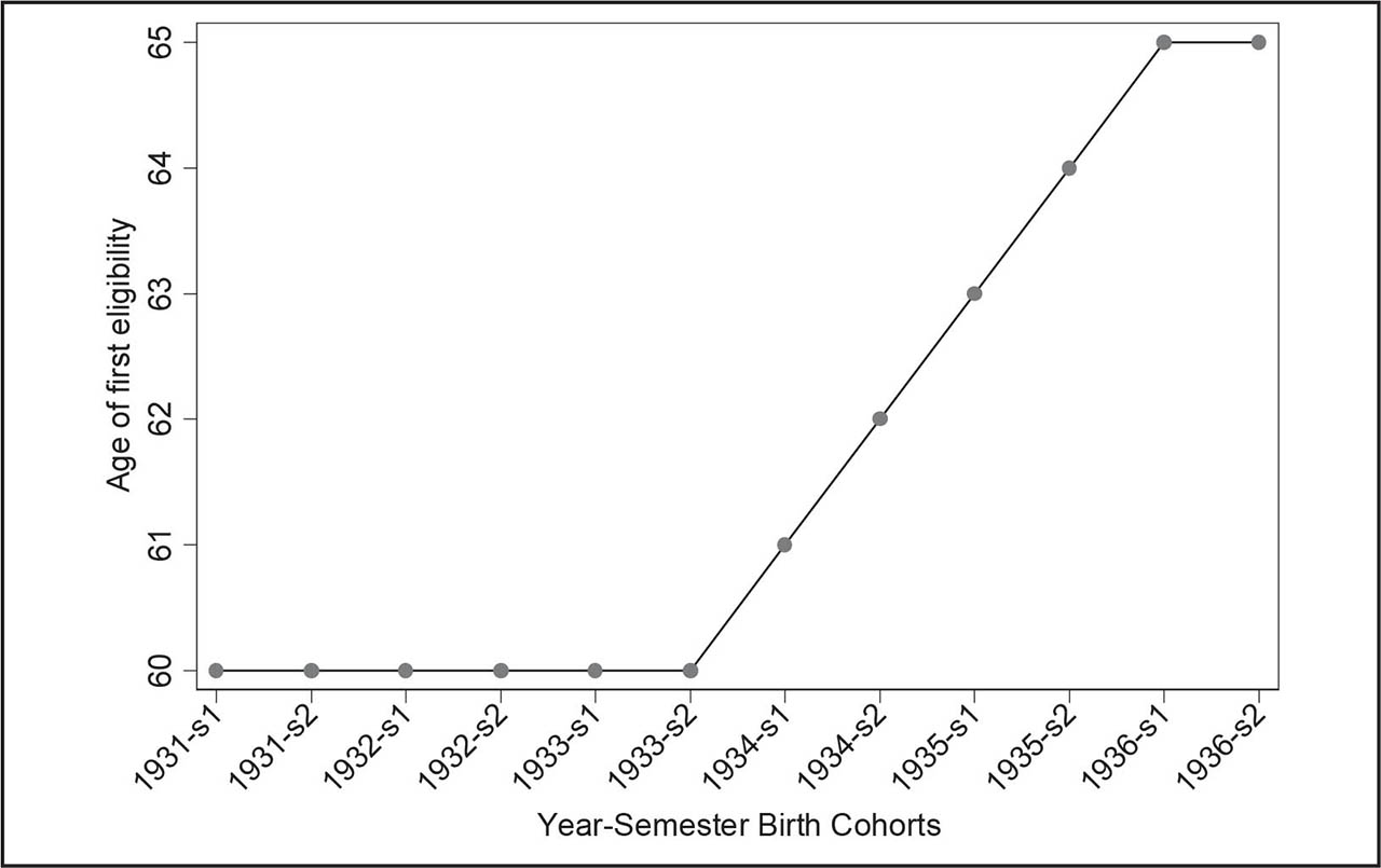
Figure 1
NRA by birth cohort as established by the 1992 Pension Reform.
Source: Author’s elaboration based on Table 1. NRA, normal retirement age.
Table 2
Sample description
| Control cohorts | Treated cohorts | |||
|---|---|---|---|---|
| Mean | St. Dev. | Mean | St. Dev. | |
| Employed (%) | 75.7 | 74.3 | ||
| Occupation (%) | ||||
| Manual | 75.4 | 74.7 | ||
| Non-manual | 14.6 | 16.1 | ||
| Manager | 0.4 | 0.7 | ||
| Self-employed | 9.6 | 8.5 | ||
| Sick-leave/work ratioa | 0.3 | 0.90 | 0.3 | 0.92 |
| Real annual earningsb | 18,072 | 13,373 | 18,980 | 13,732 |
| Panel B: Individuals characteristics at pension receipt | ||||
| Years of accrued contributions | 25.2 | 7.73 | 26.9 | 8.14 |
| Pension type | ||||
| Seniority (%) | 3.9 | 20.3 | ||
| Old-age (%) | 89.3 | 76.4 | ||
| Early retirement (%) | 6.8 | 3.3 | ||
| 2.01 | ||||
| Pension claiming age | 60.1 | 62.3 | 2.49 | |
| Individuals | 16,664 | 13,310 | ||
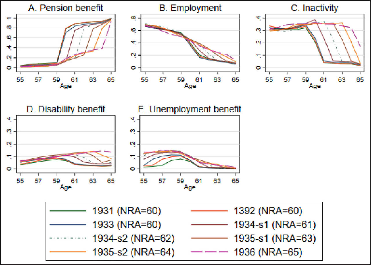
Figure 2
Labor Market Outcomes (%) by age and birth cohorts.
Notes: Proportion of persons in each labor market status by age and birth cohort. NRA, normal retirement age.
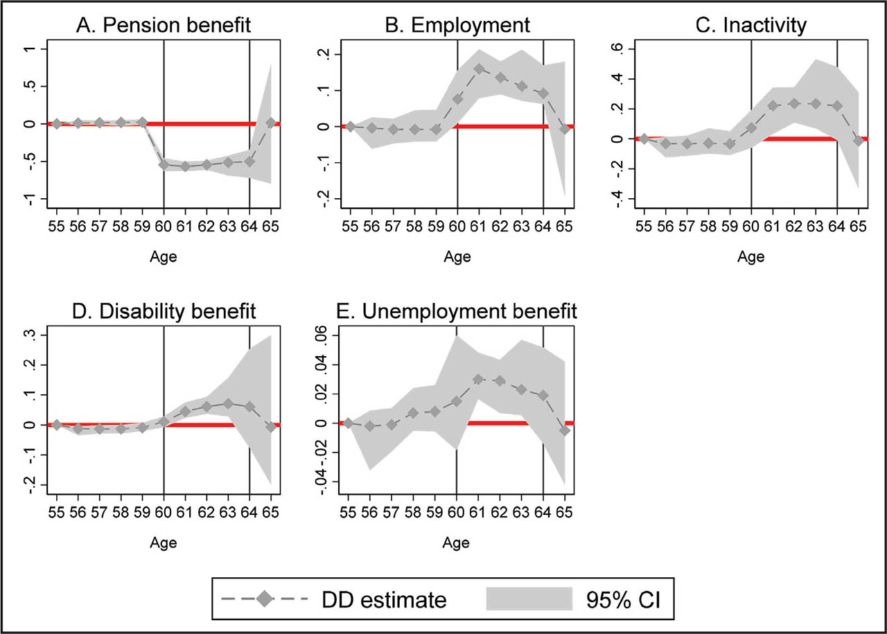
Figure 3
Effect of raising the NRA on different labor market outcomes at every single age (Ages before, during, and after the NRA rise).
Notes: The figure displays the estimated DD coefficient β (Eq. 1) and 95% CI separately for each of the outcomes. 95% CI are computed as a wild bootstrap percentile interval, thus they might be not centered around the point estimate. WB procedure with 999 repetitions. Šidàk correction for 11 multiple hypotheses. Vertical lines indicate the first (60) and last (64) treated age by the reform increasing NRA. Full output is available in Table C1 in Appendix. DD, difference-in-differences; NRA, normal retirement age; WB, wild-cluster bootstrap.
Table 3
Treated and control groups definition by age and year of birth
| Age | Control group (Ta = 0) | Treated group (Ta = 1) | Eligibility to NRA |
|---|---|---|---|
| From 55 to 59 | 1931–1933 | (1934–1936) | Placebo ages: no one is eligible |
| 60 years old | 1931–1933 | 1934–1936 | Only the control group is eligible |
| 61 years old | 1931–Jun 1934 | Jul 1934–1936 | Only the control group is eligible |
| 62 years old | 1931–Dec 1934 | 1935–1936 | Only the control group is eligible |
| 63 years old | 1931–Jun 1935 | Jul 1935–1936 | Only the control group is eligible |
| 64 years old | 1931–Dec 1935 | 1936 | Only the control group is eligible |
| 65 years old | 1931–1933 | (1934–1936) | Placebo age: everyone is eligible |
[i] Notes: Author’s elaboration based on Table 1. NRA, normal retirement age.
Table 4
Effect of raising the NRA on different labor market outcomes
| Pension benefit | Employment | Inactivity | Disability benefit | Unemployment benefit | |
|---|---|---|---|---|---|
| Panel A: Standard DD estimator | |||||
| Age<NRA | −0.440*** | 0.087*** | 0.134*** | 0.042*** | 0.016 |
| WP p-value | 0.000 | 0.000 | 0.000 | 0.000 | 0.045 |
| WB Šidàk p-value | 0.000 | 0.000 | 0.000 | 0.000 | 0.206 |
| Adj. R2 | 0.87 | 0.18 | 0.08 | 0.04 | 0.02 |
| Observations | 659,428 | 659,428 | 659,428 | 659,428 | 659,428 |
| Pre-reform mean | 0.92 | 0.12 | 0.05 | 0.02 | 0.01 |
| % change | −51% | +48% | +178% | +111% | n.s. |
| Panel B: De Chaisemartin and D’Haultfoeuille (2020b) DD estimator | |||||
| Age<NRA | −0.552*** | 0.090*** | 0.130*** | 0.025*** | 0.003 |
| WB SE | 0.016 | 0.008 | 0.005 | 0.002 | 0.005 |
Notes: The table displays the estimated DD coefficient β (Eq. 2) separately for each of the outcomes (columns). SE clustered at period level. WB procedure with 999 repetitions. Šidàk correction for five multiple hypotheses. % Change computed for coefficients significantly different from 0 with respect to pre-reform means (control cohorts at 60–64 years old). Significance based on WB p-value:
**5%,
*10% (with Šidàk correction in Panel A).
Table 5
Heterogeneous effect of rising the NRA: subsample analysis
| Pension benefit | Employment | Inactivity | Disability benefit | Unemployment benefit | Obs. | |
|---|---|---|---|---|---|---|
| Full sample | −0.440*** | 0.087*** | 0.134*** | 0.042*** | 0.016 | 659,428 |
| Always employed bef. 60 | −0.384*** | 0.092*** | 0.089*** | 0.034*** | 0.029* | 413,107 |
| Low Wage (1° tertile) | −0.459*** | 0.071*** | 0.148*** | 0.045*** | 0.022** | 135,377 |
| High wage (3° tertile) | −0.271*** | 0.075*** | 0.043*** | 0.017*** | 0.022* | 135,377 |
| Low occ. Grade (manual) | −0.414*** | 0.107*** | 0.094*** | 0.041*** | 0.034* | 299,774 |
| High occ. Grade (execut.) | −0.186 | 0.057 | 0.067 | na | −0.003 | 2,377 |
| Low health (1° tertile) | −0.423*** | 0.098* | 0.064*** | 0.078*** | 0.040* | 85,086 |
| Good health (3° tertile) | −0.377*** | 0.081*** | 0.109*** | 0.015*** | 0.014* | 255,327 |
Notes: The table displays the estimated DD coefficient β (Eq. 2) obtained from separate split sample analyses (rows) for each of the outcomes (columns). SE clustered at period level. WB procedure with 999 repetitions. Šidàk correction for five multiple hypotheses.
Significance based on WB Šidàk p-value:
DD, difference-in-differences; NRA, normal retirement age; WB, wild-cluster bootstrap.
Table 6
Heterogeneous effect of rising the NRA: fully interacted analysis
| Pension benefit | Employment | Inactivity | Disability Benefit | Unemployment benefit | |
|---|---|---|---|---|---|
| Age<NRA (Ref. categorya) | −0.167*** | 0.006 | −0.021 | 0.037*** | 0.025*** |
| Age<NRA × Low wage | −0.092*** | 0.004 | 0.056+ | −0.011 | 0.000 |
| WB p-value | 0.000 | 0.871 | 0.031 | 0.081 | 0.955 |
| WB Šidàk p-value | 0.000 | 1.000 | 0.451 | 0.288 | 1.000 |
| Age<NRA × Mid wage | −0.052*** | 0.022** | 0.009 | 0.000 | 0.003 |
| WB p-value | 0.000 | 0.005 | 0.070 | 0.957 | 0.546 |
| WB Šidàk p-value | 0.000 | 0.024 | 0.341 | 1.000 | 0.986 |
| Age<NRA × Low occ. grade | −0.18** | 0.089+ | 0.097** | −0.006 | 0.003 |
| WB p-value | 0.001 | 0.025 | 0.004 | 0.152 | 0.524 |
| WB Šidàk p-value | 0.012 | 0.242 | 0.012 | 0.545 | 0.990 |
| Age<NRA × Mid occ. grade | −0.108+ | 0.008 | 0.085* | 0.001 | 0.006 |
| WB p-value | 0.011 | 0.827 | 0.007 | 0.629 | 0.115 |
| WB Šidàk p-value | 0.130 | 1.000 | 0.064 | 0.999 | 0.561 |
| Age<NRA × Low health | −0.025* | 0.024** | −0.011 | 0.020+ | 0.007 |
| WB p-value | 0.013 | 0.003 | 0.131 | 0.017 | 0.240 |
| WB Šidàk p-value | 0.081 | 0.036 | 0.615 | 0.256 | 0.824 |
| Age<NRA × Mid health | 0.005 | 0.008 | −0.014 | 0.005 | −0.004 |
| WB p-value | 0.645 | 0.359 | 0.120 | 0.056 | 0.564 |
| WB Šidàk p-value | 0.998 | 0.921 | 0.647 | 0.390 | 0.991 |
| Adj. R2 | 0.689 | 0.62 | 0.15 | 0.055 | 0.069 |
| Observations | 371,622 | 371,622 | 371,622 | 371,622 | 371,622 |
Notes: The table displays the estimated DD coefficient β of Equation (2) interacted simultaneously with different socio-economic group indicators separately for each of the outcomes (columns).
a Ref. category composed of the three excluded categories: workers with high wage, high occupational grade (executives) and good health. SE clustered at period level. WB procedure with 999 repetitions. Šidàk correction for six multiple hypotheses.
Significance based on WB Šidàk p-value:
In addition, coefficients with WB p-value <5% are marked with +. Full output is available in Table B3 in Appendix. DD, difference-in-differences; NRA, normal retirement age; WB, wild-cluster bootstrap.
Table 7
Effect of rising ERA/NRA on different labor market outcomes: comparison of previousstudies
| Retirement benefit | Employment | Disability benefit | Unempl. benefit | Inactivity | |
|---|---|---|---|---|---|
| IT (m, NRA 60–65) (My results, Table 4) | −0.44*** | 0.087*** | 0.042*** | 0.016 | 0.134*** |
| AUT (f, NRA 60–64.5) Oguzoglu et al., 2020 (Table 2) | −0.519*** | na | 0.143*** | 0.039*** | na |
| AUS (m, ERA 60–62) Staubli and Zweimuller, 2013 (Table 3) | −0.248*** | 0.097*** | 0.010*** | 0.125*** | 0.016*** |
| GER (f, ERA, 60–62) Geyer and Welteke, 2021 (Table 1) | −0.276*** | 0.135*** | −0.007 | 0.052*** | 0.062*** |
| FRA (all, ERA 60–61) Rabaté and Rochut, 2020 (Table 5) | −0.478*** | 0.209*** | 0.059*** | 0.134*** | 0.062*** |
| UK (f, ERA 60–62) Cribb et al., 2016 (Tables 4 and 5) | −0.115*** | 0.063** | 0.040*** | 0.012*** | 0.008 |
[i] Source: Author’s elaboration.
[ii] ERA, early retirement age; NRA, normal retirement age.
Table B1
Calendar years and ages for the treated and untreated cohorts
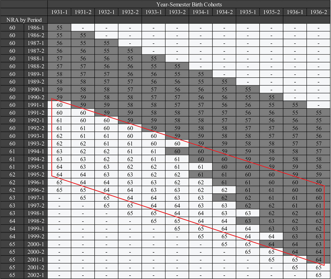
[i] Note: Each column lists the age of a given cohort in a particular semester. Each cell identifies the treatment and control groups in a particular age and period. Cells identify treatment if Age < NRA (grey color) and control if Age >= NRA (white). The composition of treated and control groups evolves with the gradual increase of NRA as shown in Table 3. For example, individuals born in the first half of 1934 (i.e., 1934-I) are “treated” only in their 60th year of age and contribute to the estimation of the effect of a rise of NRA from 60 to 61 as part of the treated group, but in the following step-wise increases (from 61 to 65) they will act as a control, as long as they had already reached NRA in 1995-I. The average DD treatment effect is identified only for the ages 60–64 (area included in the red rhombus) for which there is within and between cohort variation.
[ii] DD, difference-in-differences; NRA, normal retirement age.
Table C1
Effect of rising the NRA on different labor market outcomes at every single age (before, during, and after the NRA rise) Eq. (1)
| Pension benefit | Employment | Inactivity | Disability benefit | Unemployment benefit | |
|---|---|---|---|---|---|
| Interaction of Treated group (T) and Age dummies (Ref. Category: T X Age55) | |||||
| T × Age56 WB Šidàk p | 0.01 (0.5612) | −0.004 (1.000) | −0.032 (0.183) | −0.012 (0.000) | −0.002 (0.999) |
| T × Age57 WB Šidàk p | 0.016 (0.2853) | −0.008 (0.982) | −0.033 (0.479) | −0.013 (0.03) | −0.005 (1.000) |
| T × Age58 WB Šidàk p | 0.019 (0.5753) | −0.008 (1.000) | −0.029 (0.943) | −0.013 (0.039) | 0.007 (0.628) |
| T × Age59 WB Šidàk p | 0.022 (0.4141) | −0.008 (0.999) | −0.034 (0.854) | −0.009 (0.432) | 0.008 (0.462) |
| T × Age60 WB Šidàk p | −0.546*** (0.000) | 0.076** (0.01) | 0.073 (0.712) | 0.011 (0.571) | 0.015 (0.948) |
| T × Age61 WB Šidàk p | −0.568** (0.01) | 0.16** (0.01) | 0.221** (0.03) | 0.045*** (0.000) | 0.03*** (0.000) |
| T × Age62 WB Šidàk p | −0.546*** (0.000) | 0.136*** (0.000) | 0.236** (0.01) | 0.061*** (0.000) | 0.029** (0.01) |
| T × Age63 WB Šidàk p | −0.517** (0.01) | 0.112** (0.02) | 0.235** (0.02) | 0.071** (0.02) | 0.023** (0.039) |
| T × Age64 WB Šidàk p | −0.503*** (0.000) | 0.092*** (0.000) | 0.22* (0.059) | 0.061 (0.27) | 0.019 (0.278) |
| T × Age65 | 0.014 (0.9999) | −0.007 (1.000) | −0.014 (1.000) | −0.007 (0.999) | −0.005 (0.964) |
| Year-semester of birth dummies (Ref. Category: 1931 - I sem) | |||||
| 1931 - II sem | −0.019** | 0.040*** | 0.022 | 0.007*** | 0.005** |
| 1932 - I sem | −0.048*** | 0.070*** | 0.070*** | 0.014*** | 0.015*** |
| 1932 - II sem | −0.070*** | 0.099*** | 0.101*** | 0.010** | 0.022*** |
| 1933 - I sem | −0.123*** | 0.137*** | 0.144*** | 0.023*** | 0.028*** |
| 1933 - II sem | −0.136*** | 0.167*** | 0.171*** | 0.025*** | 0.035*** |
| 1934 - I sem | −0.193*** | 0.228*** | 0.245*** | 0.050*** | 0.054*** |
| 1934 - II sem | −0.220*** | 0.275*** | 0.277*** | 0.051*** | 0.066*** |
| 1935 - I sem | −0.257*** | 0.308*** | 0.319*** | 0.067*** | 0.072*** |
| 1935 - II sem | −0.268*** | 0.338*** | 0.353*** | 0.062*** | 0.075*** |
| 1936 - I sem | −0.278*** | 0.358*** | 0.388*** | 0.066*** | 0.080*** |
| 1936 - II sem | −0.287*** | 0.383*** | 0.420*** | 0.059*** | 0.092*** |
| Year-semester dummies (Ref. Category: 1986 - I sem) | |||||
| 1986 - II sem | 0.021*** | −0.029*** | −0.025*** | 0.003** | 0 |
| 1987 - I sem | 0.057*** | −0.101*** | −0.060*** | −0.002 | 0 |
| 1987 - II sem | 0.075*** | −0.119*** | −0.098*** | −0.002 | −0.005 |
| 1988 - I sem | 0.112*** | −0.168*** | −0.138*** | −0.004 | −0.017*** |
| 1988 - II sem | 0.134*** | −0.191*** | −0.183*** | −0.005 | −0.022*** |
| 1989 - I sem | 0.172*** | −0.246*** | −0.224*** | −0.009 | 0.023*** |
| 1989 - II sem | 0.192*** | −0.269*** | −0.268*** | −0.012 | 0.018** |
| 1990 - I sem | 0.216*** | −0.306*** | −0.302*** | −0.014 | 0.038*** |
| 1990 - II sem | 0.236*** | −0.332*** | −0.342*** | −0.017 | 0.034*** |
| 1991 - I sem | 0.254*** | −0.365*** | −0.354*** | −0.018 | 0.046*** |
| 1991 - II sem | 0.277*** | −0.397*** | −0.410*** | −0.022 | 0.045*** |
| 1992 - I sem | 0.303*** | −0.443*** | −0.436*** | −0.023 | 0.029** |
| 1992 - II sem | 0.327*** | −0.476*** | −0.474*** | −0.028 | 0.034** |
| 1993 - I sem | 0.340*** | −0.537*** | −0.495*** | −0.03 | 0.025 |
| 1993 - II sem | 0.353*** | −0.573*** | −0.531*** | −0.034 | 0.033 |
| 1994 - I sem | 0.385*** | −0.637*** | −0.576*** | −0.039 | 0.01 |
| 1994 - II sem | 0.403*** | −0.660*** | −0.593*** | −0.041 | 0.011 |
| 1995 - I sem | 0.421*** | −0.690*** | −0.602*** | −0.041 | 0 |
| 1995 - II sem | 0.439*** | −0.723*** | −0.658*** | −0.045 | −0.006 |
| 1996 - I sem | 0.461*** | −0.762*** | −0.685*** | −0.049 | −0.013 |
| 1996 - II sem | 0.480*** | −0.780*** | −0.693*** | −0.047 | −0.017 |
| 1997 - I sem | 0.514*** | −0.834*** | −0.750*** | −0.053 | −0.035 |
| 1997 - II sem | 0.535*** | −0.861*** | −0.781*** | −0.056 | −0.039 |
| 1998 - I sem | 0.551*** | −0.893*** | −0.777*** | −0.05 | −0.048 |
| 1998 - II sem | 0.581*** | −0.933*** | −0.848*** | −0.058 | −0.054 |
| 1999 - I sem | 0.608*** | −0.973*** | −0.873*** | −0.06 | −0.066** |
| 1999 - II sem | 0.616*** | −0.990*** | −0.877*** | −0.049 | −0.070** |
| 2000 - I sem | 0.652*** | −1.025*** | −0.947*** | −0.05 | −0.083** |
| 2000 - II sem | 0.677*** | −1.050*** | −0.974*** | −0.042 | −0.088** |
| 2001 - I sem | 0.679*** | −1.063*** | −0.908*** | −0.008 | −0.089** |
| 2001 - II sem | 0.672*** | −1.075*** | −0.933*** | 0.01 | −0.087** |
| 2002 - I sem | 0.742*** | −1.142*** | −1.109*** | −0.017 | −0.112*** |
| Age dummies (Reference Category: 55 years old) | |||||
| 56 | −0.038*** | 0.045*** | 0.080*** | 0.020*** | 0.013*** |
| 57 | −0.079*** | 0.091*** | 0.156*** | 0.037*** | 0.025*** |
| 58 | −0.117*** | 0.132*** | 0.234*** | 0.053*** | 0.030*** |
| 59 | −0.142*** | 0.162*** | 0.312*** | 0.064*** | 0.034*** |
| 60 | 0.483*** | 0.07 | 0.276*** | 0.059*** | 0.006 |
| 61 | 0.536*** | −0.024 | 0.180** | 0.037 | −0.030** |
| 62 | 0.529*** | 0.002 | 0.222** | 0.033 | −0.027 |
| 63 | 0.506*** | 0.043 | 0.274** | 0.033 | −0.016 |
| 64 | 0.476*** | 0.086 | 0.325*** | 0.032 | −0.003 |
| 65 | 0.503*** | 0.122 | 0.366*** | 0.038 | 0.011 |
| _cons | 0.024*** | 0.709*** | 0.331*** | 0.026*** | 0.010*** |
| Adj. R2 | 0.65 | 0.22 | 0.1 | 0.02 | 0.05 |
| Observations | 659,428 | 659,428 | 659,428 | 659,428 | 659,428 |
Notes: The table displays the regression output of Eq. (1) separately for each of the outcomes (columns). SE clustered at period level (33 groups) (sem=half year). Significance levels:
* 10%, based on: (a) WB procedure with 999 repetitions and Šidàk correction for five multiple hypotheses for the interactions terms TxAge, and (b) SE clustered for the remaining coefficients.
NRA, normal retirement age; WB, wild-cluster bootstrap.
Table C2
The average effect of raising the NRA on different labor market outcomes Eq. (2)
| Pension benefit | Employment | Inactivity | Disability Benefit | Unemployment benefit | |
|---|---|---|---|---|---|
| Age<NRA | −0.440*** | 0.087*** | 0.134*** | 0.042*** | 0.016*** |
| WB Šidàk p | (0.000) | (0.000) | (0.000) | (0.000) | (0.206) |
| Year-semester of birth dummies (Ref. Category: 1931 - I sem) | |||||
| 1931 - II sem | −0.035*** | 0.043*** | 0.027*** | 0.009*** | 0.006*** |
| 1932 - I sem | −0.079*** | 0.075*** | 0.080*** | 0.017*** | 0.016*** |
| 1932 - II sem | −0.115*** | 0.107*** | 0.116*** | 0.015*** | 0.023*** |
| 1933 - I sem | −0.187*** | 0.149*** | 0.165*** | 0.029*** | 0.030*** |
| 1933 - II sem | −0.194*** | 0.177*** | 0.189*** | 0.031*** | 0.037*** |
| 1934 - I sem | −0.269*** | 0.238*** | 0.250*** | 0.049*** | 0.057*** |
| 1934 - II sem | −0.327*** | 0.296*** | 0.295*** | 0.052*** | 0.071*** |
| 1935 - I sem | −0.390*** | 0.336*** | 0.351*** | 0.071*** | 0.078*** |
| 1935 - II sem | −0.425*** | 0.372*** | 0.398*** | 0.070*** | 0.084*** |
| 1936 - I sem | −0.478*** | 0.401*** | 0.453*** | 0.080*** | 0.090*** |
| 1936 - II sem | −0.505*** | 0.428*** | 0.490*** | 0.075*** | 0.103*** |
| Year-semester dummies (Ref. Category: 1986 - I sem) | |||||
| 1986 - II sem | 0.029*** | −0.030*** | −0.028** | 0.002 | −0.001 |
| 1987 - I sem | 0.083*** | −0.106*** | −0.066*** | −0.003 | −0.001 |
| 1987 - II sem | 0.113*** | −0.126*** | −0.106*** | −0.004 | −0.006** |
| 1988 - I sem | 0.170*** | −0.179*** | −0.153*** | −0.007 | −0.019*** |
| 1988 - II sem | 0.202*** | −0.204*** | −0.201*** | −0.009 | −0.025*** |
| 1989 - I sem | 0.257*** | −0.262*** | −0.246*** | −0.014 | 0.019*** |
| 1989 - II sem | 0.291*** | −0.288*** | −0.294*** | −0.017** | 0.013*** |
| 1990 - I sem | 0.338*** | −0.331*** | −0.343*** | −0.024** | 0.032*** |
| 1990 - II sem | 0.374*** | −0.360*** | −0.388*** | −0.029*** | 0.027*** |
| 1991 - I sem | 0.421*** | −0.399*** | −0.411*** | −0.033** | 0.037*** |
| 1991 - II sem | 0.463*** | −0.435*** | −0.472*** | −0.037*** | 0.036*** |
| 1992 - I sem | 0.513*** | −0.488*** | −0.513*** | −0.042*** | 0.021** |
| 1992 - II sem | 0.555*** | −0.526*** | −0.561*** | −0.050*** | 0.024** |
| 1993 - I sem | 0.589*** | −0.593*** | −0.593*** | −0.055*** | 0.016 |
| 1993 - II sem | 0.619*** | −0.633*** | −0.638*** | −0.062*** | 0.023*** |
| 1994 - I sem | 0.691*** | −0.708*** | −0.703*** | −0.074*** | −0.002 |
| 1994 - II sem | 0.678*** | −0.727*** | −0.720*** | −0.077*** | 0.001 |
| 1995 - I sem | 0.709*** | −0.758*** | −0.730*** | −0.077*** | −0.012 |
| 1995 - II sem | 0.772*** | −0.796*** | −0.797*** | −0.086*** | −0.019 |
| 1996 - I sem | 0.756*** | −0.822*** | −0.801*** | −0.085*** | −0.024** |
| 1996 - II sem | 0.789*** | −0.842*** | −0.812*** | −0.084*** | −0.028** |
| 1997 - I sem | 0.870*** | −0.901*** | −0.872*** | −0.092*** | −0.047*** |
| 1997 - II sem | 0.864*** | −0.919*** | −0.885*** | −0.090*** | −0.049*** |
| 1998 - I sem | 0.904*** | −0.957*** | −0.888*** | −0.085*** | −0.059*** |
| 1998 - II sem | 1.007*** | −1.013*** | −0.974*** | −0.096*** | −0.067*** |
| 1999 - I sem | 0.992*** | −1.046*** | −0.979*** | −0.092*** | −0.080*** |
| 1999 - II sem | 1.028*** | −1.071*** | −0.994*** | −0.082*** | −0.086*** |
| 2000 - I sem | 1.171*** | −1.131*** | −1.093*** | −0.093*** | −0.104*** |
| 2000 - II sem | 1.130*** | −1.146*** | −1.095*** | −0.079** | −0.107*** |
| 2001 - I sem | 1.166*** | −1.166*** | −1.051*** | −0.051 | −0.110*** |
| 2001 - II sem | 1.212*** | −1.188*** | −1.113*** | −0.043 | −0.112*** |
| 2002 - I sem | 1.277*** | −1.249*** | −1.278*** | −0.064** | −0.132*** |
| Age dummies (Reference Category: 55 years old) | |||||
| 56 | −0.069*** | 0.051*** | 0.082*** | 0.019*** | 0.014*** |
| 57 | −0.146*** | 0.105*** | 0.174*** | 0.040*** | 0.028*** |
| 58 | −0.220*** | 0.154*** | 0.271*** | 0.062*** | 0.038*** |
| 59 | −0.282*** | 0.194*** | 0.369*** | 0.080*** | 0.043*** |
| 60 | −0.165** | 0.189*** | 0.459*** | 0.110*** | 0.027*** |
| 61 | −0.134 | 0.130*** | 0.430*** | 0.106*** | −0.003 |
| 62 | −0.158 | 0.150*** | 0.476*** | 0.109*** | −0.001 |
| 63 | −0.189** | 0.184*** | 0.521*** | 0.110*** | 0.009 |
| 64 | −0.244** | 0.227*** | 0.563*** | 0.106*** | 0.022 |
| 65 | −0.254** | 0.270*** | 0.599*** | 0.111*** | 0.037** |
| _cons | 0.464*** | 0.622*** | 0.197*** | −0.015*** | −0.005 |
| Adj. R2 | 0.64 | 0.22 | 0.1 | 0.02 | 0.05 |
| Observations | 659,428 | 659,428 | 659,428 | 659,428 | 659,428 |
Notes: The table displays the regression output of Eq. (2) separately for each of the outcomes (columns). SE clustered at period level (33 groups) (sem=half year). Significance levels:
* 10%, based on: (a) WB procedure with 999 repetitions and Šidàk correction for five multiple hypotheses for the indicator terms Age<NRA, and (b) SE clustered for the remaining coefficients.
NRA, normal retirement age; WB, wild-cluster bootstrap.
Table C3
Heterogeneous effect of rising the NRA: fully interacted analysis (based on Eq. (2))
| Pension benefit | Employment | Inactivity | Disability benefit | Unemployment benefit | |
|---|---|---|---|---|---|
| Age<NRA (Ref. Categorya) | −0.167*** | 0.006 | −0.021 | 0.037*** | 0.025*** |
| Age<NRA × Low wage | −0.092*** | 0.004 | 0.056 | −0.011 | 0 |
| WP p | 0.000 | 0.871 | 0.031 | 0.081 | 0.955 |
| WP p Šidàk correction | 0.000 | 1.000 | 0.451 | 0.288 | 1.000 |
| Age<NRA × Mid wage | −0.052*** | 0.022** | 0.009 | 0 | 0.003 |
| WP p | 0.000 | 0.005 | 0.070 | 0.957 | 0.546 |
| WP p Šidàk correction | 0.000 | 0.024 | 0.341 | 1.000 | 0.986 |
| Age<NRA × Low occ. Grade | −0.180** | 0.089+ | 0.097** | −0.006 | 0.003 |
| WP p | 0.001 | 0.025 | 0.004 | 0.152 | 0.524 |
| WP p Šidàk correction | 0.012 | 0.242 | 0.012 | 0.545 | 0.990 |
| Age<NRA × Mid occ. Grade | −0.108 | 0.008 | 0.085* | 0.001 | 0.006 |
| WP p | 0.011 | 0.827 | 0.007 | 0.629 | 0.115 |
| WP p Šidàk correction | 0.130 | 1.000 | 0.064 | 0.999 | 0.561 |
| Age<NRA × Low health | −0.025* | 0.024** | −0.011 | 0.020+ | 0.007 |
| WP p | 0.013 | 0.003 | 0.131 | 0.017 | 0.240 |
| WP p Šidàk correction | 0.081 | 0.036 | 0.615 | 0.256 | 0.824 |
| Age<NRA × Mid health | 0.005 | 0.008 | −0.014 | 0.005 | −0.004 |
| WP p | 0.645 | 0.359 | 0.120 | 0.056 | 0.564 |
| WP p Šidàk correction | 0.998 | 0.921 | 0.647 | 0.390 | 0.991 |
| Year-semester of birth dummies (Ref. Category: 1931 - I sem) | |||||
| 1931 - II sem | −0.037*** | 0.049*** | 0.033*** | 0.008*** | 0.010*** |
| 1932 - I sem | −0.075*** | 0.099*** | 0.068*** | 0.011*** | 0.024*** |
| 1932 - II sem | −0.124*** | 0.141*** | 0.105*** | 0.018*** | 0.033*** |
| 1933 - I sem | −0.198*** | 0.199*** | 0.141*** | 0.026*** | 0.046*** |
| 1933 - II sem | −0.200*** | 0.225*** | 0.162*** | 0.029*** | 0.051*** |
| 1934 - I sem | −0.292*** | 0.324*** | 0.216*** | 0.044*** | 0.075*** |
| 1934 - II sem | −0.350*** | 0.376*** | 0.263*** | 0.053*** | 0.085*** |
| 1935 - I sem | −0.421*** | 0.456*** | 0.305*** | 0.065*** | 0.103*** |
| 1935 - II sem | −0.456*** | 0.500*** | 0.351*** | 0.073*** | 0.111*** |
| 1936 - I sem | −0.515*** | 0.561*** | 0.389*** | 0.081*** | 0.122*** |
| 1936 - II sem | −0.534*** | 0.591*** | 0.425*** | 0.076*** | 0.134*** |
| Year-semester dummies (Ref. Category: 1986 - I sem) | |||||
| 1986 - II sem | 0.017 | −0.024 | −0.014 | −0.003 | −0.005 |
| 1987 - I sem | 0.069*** | −0.087*** | −0.055*** | −0.012*** | −0.020*** |
| 1987 - II sem | 0.105*** | −0.126*** | −0.083*** | −0.017*** | −0.030*** |
| 1988 - I sem | 0.164*** | −0.186*** | −0.124*** | −0.027*** | −0.044*** |
| 1988 - II sem | 0.200*** | −0.226*** | −0.152*** | −0.033*** | −0.053*** |
| 1989 - I sem | 0.257*** | −0.291*** | −0.194*** | −0.042*** | −0.068*** |
| 1989 - II sem | 0.301*** | −0.339*** | −0.227*** | −0.050*** | −0.079*** |
| 1990 - I sem | 0.359*** | −0.405*** | −0.271*** | −0.059*** | −0.093*** |
| 1990 - II sem | 0.403*** | −0.454*** | −0.306*** | −0.067*** | −0.104*** |
| 1991 - I sem | 0.464*** | −0.491*** | −0.332*** | −0.074*** | −0.118*** |
| 1991 - II sem | 0.521*** | −0.559*** | −0.386*** | −0.082*** | −0.124*** |
| 1992 - I sem | 0.578*** | −0.632*** | −0.427*** | −0.090*** | −0.151*** |
| 1992 - II sem | 0.626*** | −0.680*** | −0.472*** | −0.099*** | −0.148*** |
| 1993 - I sem | 0.660*** | −0.751*** | −0.501*** | −0.108*** | −0.171*** |
| 1993 - II sem | 0.689*** | −0.802*** | −0.541*** | −0.116*** | −0.167*** |
| 1994 - I sem | 0.757*** | −0.887*** | −0.597*** | −0.128*** | −0.199*** |
| 1994 - II sem | 0.737*** | −0.904*** | −0.611*** | −0.131*** | −0.195*** |
| 1995 - I sem | 0.772*** | −0.938*** | −0.622*** | −0.133*** | −0.208*** |
| 1995 - II sem | 0.835*** | −0.993*** | −0.676*** | −0.143*** | −0.221*** |
| 1996 - I sem | 0.825*** | −1.025*** | −0.685*** | −0.146*** | −0.228*** |
| 1996 - II sem | 0.866*** | −1.053*** | −0.698*** | −0.146*** | −0.231*** |
| 1997 - I sem | 0.947*** | −1.129*** | −0.749*** | −0.154*** | −0.259*** |
| 1997 - II sem | 0.948*** | −1.153*** | −0.765*** | −0.155*** | −0.261*** |
| 1998 - I sem | 0.993*** | −1.201*** | −0.770*** | −0.152*** | −0.275*** |
| 1998 - II sem | 1.092*** | −1.274*** | −0.838*** | −0.163*** | −0.288*** |
| 1999 - I sem | 1.089*** | −1.319*** | −0.846*** | −0.162*** | −0.303*** |
| 1999 - II sem | 1.129*** | −1.357*** | −0.865*** | −0.155*** | −0.310*** |
| 2000 - I sem | 1.268*** | −1.439*** | −0.941*** | −0.169*** | −0.336*** |
| 2000 - II sem | 1.246*** | −1.470*** | −0.949*** | −0.161*** | −0.341*** |
| 2001 - I sem | 1.285*** | −1.498*** | −0.921*** | −0.136*** | −0.344*** |
| 2001 - II sem | 1.326*** | −1.545*** | −0.969*** | −0.136*** | −0.344*** |
| 2002 - I sem | 1.386*** | −1.627*** | −1.099*** | −0.149*** | −0.369*** |
| Age dummies (Reference Category: 55 years old) | |||||
| 56 | −0.099*** | 0.106*** | 0.074*** | 0.016*** | 0.024*** |
| 57 | −0.198*** | 0.216*** | 0.151*** | 0.033*** | 0.049*** |
| 58 | −0.293*** | 0.329*** | 0.228*** | 0.050*** | 0.074*** |
| 59 | −0.381*** | 0.437*** | 0.303*** | 0.066*** | 0.097*** |
| 60 | −0.152 | 0.123*** | 0.595*** | 0.160*** | 0.250*** |
| 61 | −0.111 | 0.021 | 0.595*** | 0.163*** | 0.212*** |
| 62 | −0.125 | 0.035 | 0.641*** | 0.170*** | 0.216*** |
| 63 | −0.158 | 0.074** | 0.684*** | 0.175*** | 0.229*** |
| 64 | −0.219 | 0.131*** | 0.725*** | 0.176*** | 0.247*** |
| 65 | −0.255 | 0.192*** | 0.764*** | 0.185*** | 0.268*** |
| _cons | 0.126** | 1.033*** | 0.04 | −0.068*** | −0.051*** |
| Adj. R2 | 0.69 | 0.62 | 0.15 | 0.05 | 0.07 |
| Observations | 371,622 | 371,622 | 371,622 | 371,622 | 371,622 |
Notes: The table displays the estimated DD coefficient β of Eq. (2) interacted simultaneously with different socio-economic group indicators separately for each of the outcomes (columns).
a Ref. category composed of the three excluded categories: workers with high wage, high occupational grade (executives), and good health. SE clustered at period level with WB procedure with 999 repetitions. Šidàk correction for six multiple hypotheses.
Significance levels:
* 10%, based on: (a) WB procedure with 999 repetitions and Šidàk correction for six multiple hypotheses for the term Age<NRA interacted with socio-economic group indicators, and (b) SE clustered for the remaining coefficients.
DD, difference-in-differences; NRA, normal retirement age; WB, wild-cluster bootstrap.
Table D1
Effect of raising the NRA: Eq. 2 controlling also for Individual Fixed Effects
| Pension benefit | Employment | Inactivity | Disability benefit | Unemployment benefit | |
|---|---|---|---|---|---|
| Age<NRA | −0.440*** | 0.087*** | 0.134*** | 0.042*** | 0.016 |
| WB p | 0.000 | 0.000 | 0.000 | 0.000 | 0.045 |
| WB Šidàk p | 0.000 | 0.000 | 0.000 | 0.000 | 0.206 |
| Adj. R2 | 0.77 | 0.61 | 0.54 | 0.63 | 0.35 |
| Observations | 659,428 | 659,428 | 659,428 | 659,428 | 659,428 |
Notes: The table displays the estimated DD coefficient β of Eq. (2) separately for each of the outcomes (columns). Controls include all those specified in Eq. (2) plus individuals fixed effects. SE clustered at period level. WB procedure with 999 repetitions. Significance legend based on WB p-value corrected for five multiple hypotheses:
DD, difference-in-differences; NRA, normal retirement age; WB, wild-cluster bootstrap.
Table D2
Effect of raising the NRA: Eq. 2 excluding from controls time fixed effects
| Pension benefit | Employment | Inactivity | Disability benefit | Unemployment benefit | |
|---|---|---|---|---|---|
| Age<NRA | −0.454*** | 0.090** | 0.161** | 0.043*** | −0.019* |
| WB p | 0.000 | 0.007 | 0.002 | 0.000 | 0.016 |
| WB Šidàk p | 0.000 | 0.035 | 0.010 | 0.000 | 0.070 |
| Adj. R2 | 0.77 | 0.61 | 0.54 | 0.63 | 0.35 |
| Observations | 659,428 | 659,428 | 659,428 | 659,428 | 659,428 |
Notes: The table displays the estimated DD coefficient β of Eq. (2) separately for each of the outcomes (columns). Controls include all those specified in Eq. (2) except for time-fixed effects. SE clustered at period level. WB procedure with 999 repetitions. Significance legend based on WB p-value corrected for five multiple hypotheses:
DD, difference-in-differences; NRA, normal retirement age; WB, wild-cluster bootstrap.
Table D3
Effect of raising the NRA: Eq. 2 excluding years 1992–1993
| Pension benefit | Employment | Inactivity | Disability benefit | Unemployment benefit | |
|---|---|---|---|---|---|
| Age<NRA | −0.417*** | 0.078*** | 0.127*** | 0.043*** | 0.015 |
| WB p | 0.000 | 0.004 | 0.004 | 0.000 | 0.047 |
| WB Šidàk p | 0.000 | 0.020 | 0.020 | 0.000 | 0.214 |
| Adj. R2 | 0.64 | 0.24 0.1 | 0.02 | 0.05 | |
| Observations | 539,532 | 539,532 | 539,532 | 539,532 | 539,532 |
Notes: The table displays the estimated DD coefficient β of Eq. (2) separately for each of the outcomes (columns). Controls include all those specified in Eq. (2). Years 1992–1993 excluded from the analysis. SE clustered at period level. WB procedure with 999 repetitions. Significance legend based on WB p-value corrected for five multiple hypotheses:
DD, difference-in-differences; NRA, normal retirement age; WB, wild-cluster bootstrap.
Table D4
Effect of raising the NRA: Eq. 2 excluding individuals with < 15 years of contributions in 1992
| Pension benefit | Employment | Inactivity | Disability benefit | Unemployment benefit | |
|---|---|---|---|---|---|
| Age<NRA | −0.440*** | 0.087*** | 0.133*** | 0.042*** | 0.016** |
| WB p | 0.000 | 0.000 | 0.000 | 0.000 | 0.001 |
| WB Šidàk p | 0.000 | 0.000 | 0.000 | 0.000 | 0.005 |
| Adj. R2 | 0.64 | 0.22 | 0.1 | 0.02 | 0.05 |
| Observations | 657,756 | 657,756 | 657,756 | 657,756 | 657,756 |
Notes: The table displays the estimated DD coefficient β of Eq. (2) separately for each of the outcomes (columns). SE clustered at period level. WB procedure with 999 repetitions. Significance based on WB p-value corrected for five multiple hypotheses:
DD, difference-in-differences; NRA, normal retirement age; WB, wild-cluster bootstrap.
Table D5
Change in the pension base (average of last N years of wages before pension claiming)
| N Years | Avg. Annual Wage over N years | % change from N to N+1 |
|---|---|---|
| 5 | 24,905.47 | |
| 6 | 24,832.08 | −0.3% |
| 7 | 24,752.02 | −0.3% |
| 8 | 24,696.57 | −0.2% |
| 9 | 24,663.13 | −0.1% |
| 10 | 24,631.77 | −0.1% |
[i] Note: Author’s calculation on the final sample of analysis using WHIP data.
[ii] WHIP, Working Histories Italian Panel.
Table D6
Effect of raising the NRA on Old-age pension and Early pension types (Eq. 2)
| Old age pension benefits | Early pension benefits | |
|---|---|---|
| Age<NRA | −0.549*** | −0.025 |
| WB p | 0.000 | 0.379 |
| WB Šidàk p | 0.000 | 0.907 |
| Adj. R2 | 0.75 | 0.51 |
| Observations | 551,034 | 108,394 |
Notes: The table displays the estimated DD coefficient β of Eq. (2) separately for the outcomes “Old-age Pension” and “Early Pension” which includes both seniority pension and other early pension options. Controls include all those specified in Eq. (2). SE clustered at period level. WB procedure with 999 repetitions. Significance legend based on WB p-value corrected for two multiple hypotheses:
DD, difference-in-differences; NRA, normal retirement age; WB, wild-cluster bootstrap.
Table D7
Heterogeneous Effect of rising the NRA: fully interacted analysis using characteristics measure at 55 years vs 55–59 years
| Panel A: Characteristics measured at 55 years | Panel B: Characteristics measured at 55 – 59 years | |||||||||
|---|---|---|---|---|---|---|---|---|---|---|
| Pension Benefit | Employment | Inactivity | Disability benefit | Unemployment benefit | Pension benefit | Employment | Inactivity | Disability benefit | Unemployment benefit | |
| Age<NRA (Ref. cat.a) | −0.166** | 0.011 | −0.025 | 0.036*** | 0.019 | −0.170* | 0.015 | −0.024 | 0.038*** | 0.025*** |
| WP p | 0.001 | 0.713 | 0.419 | 0.000 | 0.071 | 0.012 | 0.693 | 0.441 | 0.000 | 0.000 |
| WP p Šidàk correction | 0.020 | 0.998 | 0.943 | 0.000 | 0.373 | 0.059 | 0.997 | 0.946 | 0 | 0.000 |
| Age<NRA × Low wage | −0.121*** | 0.021 | 0.051+ | −0.004 | −0.007*** | −0.090*** | 0.000 | 0.057+ | −0.012+ | 0.002 |
| WP p | 0.001 | 0.126 | 0.031 | 0.420 | 0.002 | 0.000 | 0.995 | 0.050 | 0.033 | 0.331 |
| WP p Šidàk correction | 0.000 | 0.590 | 0.274 | 0.932 | 0.005 | 0.000 | 1.000 | 0.226 | 0.155 | 0.866 |
| Age<NRA × Mid wage | −0.068*** | 0.027* | 0.012 | 0.004 | −0.001 | −0.052*** | 0.022** | 0.009+ | 0.000 | 0.003 |
| WP p | 0.000 | 0.012 | 0.070 | 0.241 | 0.887 | 0.000 | 0.006 | 0.047 | 0.880 | 0.600 |
| WP p Šidàk correction | 0.000 | 0.059 | 0.327 | 0.753 | 1.000 | 0.000 | 0.030 | 0.214 | 1 | 0.990 |
| Age<NRA × Low occ. grade | −0.162** | 0.085+ | 0.091* | 0.001 | 0.017+ | −0.179** | 0.092+ | 0.090* | 0.003 | 0.005 |
| WP p | 0.001 | 0.023 | 0.011 | 0.452 | 0.049 | 0.006 | 0.035 | 0.016 | 0.062 | 0.453 |
| WP p Šidàk correction | 0.039 | 0.110 | 0.078 | 0.919 | 0.278 | 0.030 | 0.163 | 0.078 | 0.274 | 0.9508 |
| Age<NRA × Mid occ. grade | −0.099* | 0.000 | 0.086* | 0.004 | 0.015 | −0.104+ | 0.003 | 0.085* | 0.002 | 0.007 |
| WP p | 0.007 | 0.988 | 0.012 | 0.108 | 0.102 | 0.029 | 0.950 | 0.011 | 0.362 | 0.145 |
| WP p Šidàk correction | 0.054 | 1.000 | 0.068 | 0.436 | 0.278 | 0.137 | 1 | 0.054 | 0.895 | 0.5435 |
| R2-adjusted | 0.70 | 0.62 | 0.13 | 0.05 | 0.07 | 0.69 | 0.62 | 0.14 | 0.05 | 0.07 |
| Nobservations | 352,576 | 352,576 | 352,576 | 352,576 | 352,576 | 352,576 | 352,576 | 352,576 | 352,576 | 352,576 |
Notes: The table displays the estimated DD coefficient β of Eq. (2) interacted simultaneously with different socio-economic group indicators separately for each of the outcomes (columns).
a Ref. category composed of the two excluded categories: workers with high wage and high occupational grade (executives). SE clustered at period level with WB procedure with 999 repetitions. Šidàk correction for five multiple hypotheses. Significance level based on WB p-value with Šidàk correction:
DD, difference-in-differences; NRA, normal retirement age; WB, wild-cluster bootstrap.