
Table 1
Summary of parameters in our model
| Parameter | Interpretation | ||
|---|---|---|---|
| 0. | The wage differential between linked and nonlinked hires, controlling for only observed worker and firm characteristics. | ||
| 1. | The wage differential between linked and nonlinked hires, controlling for unobserved firm and worker heterogeneity (but not match heterogeneity). | ||
| 1a. | θ | The pure ‘presence effects’ of having a potential referrer at the firm. | |
| 1b. | Bias arising from the possibility that linked workers are better matched with firms (match selection). | ||
| 2. | The average worker effect differential between linked and nonlinked hires. | ||
| 2a. | The average worker effect differentials between linked and nonlinked hires within firms. | ||
| 2b. | The average worker effect differential between firms that tend to make linked hires and those that tend to make nonlinked hires. | ||
| 3. | The average firm effect differential between linked and nonlinked hires. | ||
| 3a. | The average firm effect differentials between linked and nonlinked hires within worker careers. | ||
| 3b. | The average firm effect differential between workers that tend to be hired with and without links. |
[i] Note: also contains the expected difference in error terms from Eq. (1), controlling for observables and person and firm effects. Our identifying assumption is that this term is zero. Also could contain additional differences in the error terms due to misspecification or proxy issues that are only relevant if one does not control for two-way fixed effects. This is also assumed to be zero. This way and .
Table 2
Summary statistics: job entrants, freshly acquired jobs, and receiving firms
| Subsample | Nonlinked subgroups | Control group | |||||
|---|---|---|---|---|---|---|---|
| Linked | Nonlinked | First spell | W/o small firm experience | Control group | Always nonlinked | Nonlinked and linked | |
| No. of observations | 20,227 | 944,579 | 135,818 | 147,600 | 661,161 | 645,253 | 15,908 |
| Log of relative daily earnings | −0.470 | −0.580 | −0.745 | −0.468 | −0.571 | −0.572 | −0.552 |
| Monthly earnings (HUF) | 128,511 | 108,053 | 80,897 | 127,616 | 109,264 | 109,245 | 110,046 |
| Age | 38.0 | 32.7 | 25.6 | 32.3 | 34.2 | 34.2 | 36.2 |
| Elementary education | 12% | 11% | 21% | 14% | 9% | 9% | 13% |
| Secondary education | 63% | 66% | 63% | 65% | 67% | 67% | 64% |
| Tertiary education | 25% | 23% | 16% | 22% | 25% | 25% | 24% |
| Central Hungary | 32% | 34% | 34% | 29% | 35% | 35% | 34% |
| Central Transdanubia | 12% | 12% | 10% | 15% | 12% | 12% | 13% |
| Western Transdanubia | 9% | 10% | 8% | 12% | 10% | 10% | 9% |
| Southern Transdanubia | 8% | 7% | 6% | 8% | 8% | 8% | 8% |
| Northern Hungary | 11% | 9% | 8% | 10% | 9% | 9% | 11% |
| Northern Great Plain | 13% | 11% | 11% | 13% | 11% | 11% | 12% |
| Southern Great Plain | 12% | 11% | 10% | 10% | 11% | 11% | 11% |
| Max. number of workplaces | 5.39 | 5.57 | 2.58 | 4.77 | 6.37 | 6.35 | 7.27 |
| Occupation specific experience | 70% | 47% | – | 37% | 59% | 59% | 69% |
| Length of prev. unemployment | 1.5 | 2.2 | – | 2.4 | 2.1 | 2.2 | 1.6 |
| Manager | 7% | 3% | 2% | 4% | 4% | 4% | 5% |
| White-collar work | 6% | 6% | 6% | 8% | 6% | 6% | 5% |
| Other white-collar work | 16% | 19% | 24% | 20% | 18% | 18% | 14% |
| Skilled blue-collar work | 43% | 40% | 38% | 34% | 41% | 41% | 44% |
| Unskilled blue-collar work | 28% | 31% | 30% | 35% | 30% | 30% | 33% |
| Relative wage level of firm | 0.907 | 0.877 | 0.816 | 1.028 | 0.856 | 0.857 | 0.815 |
| Sector: Agriculture | 3% | 2% | 3% | 2% | 2% | 2% | 2% |
| Sector: Industry | 41% | 34% | 32% | 38% | 34% | 34% | 36% |
| Sector: Trade and services | 56% | 64% | 65% | 60% | 64% | 64% | 62% |
| Foreign firm | 18% | 20% | 20% | 27% | 19% | 19% | 16% |
| Domestic firm | 82% | 80% | 80% | 73% | 81% | 81% | 84% |
| Number of employees | 39.2 | 42.9 | 44.4 | 60.0 | 38.8 | 39.0 | 30.8 |
[i] Note: The estimation sample consists of starting months of worker employment spells, between 2006 and 2011, which follow a maximum 12-month long job-search period. It includes those 15–65 years old, private sector employees, who had less than 15 distinct employment spells in the observation period and did not receive social transfers. The table comprises the average wage outcomes of individuals upon entry to a new firm, demonstrates the personal traits of workers, and contains the characteristics of the workers’ new jobs and firms. Indented figures reflect statistically significant differences (p < 0.05) from the linked group, according to t-tests.
Table 3
Decomposition of co-worker gains by gender
| Male | 0.0465*** (0.0055) | 0.0213*** (0.0051) | 0.0167*** (0.0038) | 0.0086* (0.0041) | 0.0125*** (0.0034) | 0.0118* (0.0049) | 0.0041 (0.0023) | −0.0032 (0.0034) |
| Female | 0.0313*** (0.0082) | −0.0024 (0.0096) | 0.0254*** (0.0063) | 0.0083 (0.0064) | 0.0265*** (0.0055) | 0.0148 (0.0080) | −0.0010 (0.0038) | −0.0065 (0.0057) |
| N | 964,806 | 501,200 | 964,806 | 964,806 | 943,643 | 571,441 | 964,806 | 964,806 |
| Ni | 616,386 | 197,435 | 616,386 | 616,386 | 616,365 | 223,021 | 616,386 | 616,386 |
| Nj | 105,818 | 61,121 | 105,818 | 105,818 | 84,655 | 105,778 | 105,818 | 105,818 |
| R2 | 0.327 | 0.860 | 0.204 | 0.200 | 0.453 | 0.612 | 0.052 | 0.087 |
[i] Note: Estimation results from the main regression on the logarithm of daily earnings upon job entry (Eq. (7)), without any and with two-way fixed effects, and the consecutive decomposition regressions on estimated firm and individual effects (Eqs (8-13)), respectively. The selection parameters in the columns reflect overall, within unit and between unit differences in individual and firm effects, respectively. Our variable of interest, the proxy for links, is interacted with two gender categories. Additional controls (if the corresponding fixed effects are not included) consist of gender, quadratic age interacted with imputed education, residence, the number of workplaces and job search length in an elastic form, five levels of occupation, two-digit industry codes, firm ownership, a dummy for occupation-specific experience, and dummies for calendar years. All controls are interacted with the indicators for first employment spells and for nonlinked workers without small firm experience. These observations contribute only to the proper estimation of firm effects. Standard errors are in parentheses and clustered at both firm level and individual level. *Statistically significant at 0.05 level; **at 0.01 level; and ***at 0.001 level.
Table 4
Decomposition of co-worker gains by occupations—male results
| Manager | −0.0988*** (0.0259) | −0.0030 (0.0310) | −0.0775*** (0.0211) | −0.0183 (0.0142) | −0.0699*** (0.0196) | 0.0226 (0.0241) | −0.0076 (0.0092) | −0.0409** (0.0127) |
| SkilledW | 0.0924*** (0.0274) | 0.0551* (0.0235) | −0.0006 (0.0187) | 0.0378* (0.0179) | −0.0049 (0.0169) | 0.0094 (0.0250) | 0.0044 (0.0101) | 0.0285 (0.0156) |
| UnskilledW | 0.0627*** (0.0182) | 0.0409* (0.0183) | 0.0167 (0.0134) | 0.0051 (0.0129) | 0.0153 (0.0120) | −0.0113 (0.0172) | 0.0013 (0.0076) | 0.0164 (0.0108) |
| SkilledB | 0.0584*** (0.0070) | 0.0228** (0.0077) | 0.0217*** (0.0050) | 0.0140* (0.0055) | 0.0128** (0.0044) | 0.0123 (0.0065) | 0.0089** (0.0034) | 0.0016 (0.0047) |
| UnskilledB | 0.0475*** (0.0081) | 0.0118 (0.0075) | 0.0340*** (0.0048) | 0.0017 (0.0069) | 0.0326*** (0.0045) | 0.0161 (0.0085) | 0.0014 (0.0030) | −0.0144* (0.0056) |
| N | 964,806 | 501,200 | 964,806 | 964,806 | 943,643 | 571,442 | 964,806 | 964,806 |
| Ni | 616,386 | 197,435 | 616,386 | 616,386 | 616,365 | 223,021 | 616,386 | 616,386 |
| Nj | 105,818 | 61,121 | 105,818 | 105,818 | 84,655 | 105,778 | 105,818 | 105,818 |
| R2 | 0.327 | 0.860 | 0.190 | 0.200 | 0.443 | 0.612 | 0.052 | 0.086 |
[i] Note: Estimation results from the main regression on the logarithm of daily earnings upon job entry (Eq. (7)), without any and with two-way fixed effects, and the consecutive decomposition regressions on estimated firm and individual effects (Eqs (8–13)), respectively. The selection parameters in the columns reflect overall, within unit and between unit differences in individual and firm effects, respectively. Our variable of interest, the proxy for links, is interacted with 10 categories based on gender and five occupational categories: managers, skilled white-collar, unskilled white-collar, skilled blue-collar, and unskilled blue-collar workers. Only the parameters for male workers are presented. For the list of additional controls, see Table 3. Standard errors are in parentheses and clustered at both firm level and individual level.
*Statistically significant at 0.05 level; **at 0.01 level; ***at 0.001 level.
Table 5
Endogenous and exogenous job mobility
| Endog. | 0.0436*** (0.0058) | 0.0162** (0.0055) | 0.0188*** (0.0041) | 0.0086* (0.0044) | 0.0161*** (0.0037) | 0.0071 (0.0054) | 0.0027 (0.0025) | 0.0015 (0.0037) |
| Exog. | 0.0620*** (0.0119) | 0.0423*** (0.0117) | 0.0103 (0.0080) | 0.0095 (0.0087) | −0.0003 (0.0072) | 0.0366*** (0.0107) | 0.0106** (0.0041) | −0.0272*** (0.0073) |
| N | 964,806 | 501,200 | 964,806 | 964,806 | 943,643 | 571,442 | 964,806 | 964,806 |
| Ni | 616,386 | 197,435 | 616,386 | 616,386 | 616,365 | 223,021 | 616,386 | 616,386 |
| Nj | 105,818 | 61,121 | 105,818 | 105,818 | 84,655 | 105,778 | 105,818 | 105,818 |
| R2 | 0.327 | 0.860 | 0.203 | 0.200 | 0.453 | 0.612 | 0.052 | 0.087 |
[i] Note: Estimation results from the main regression on the logarithm of daily earnings upon job entry (Eq. (7)), without any and with two-way fixed effects, and the consecutive decomposition regressions on estimated firm and individual effects (Eqs (8-13)), respectively. The selection parameters in the columns reflect overall, within unit and between unit differences in individual and firm effects, respectively. Our variable of interest, the proxy for links, is interacted with four categories based on gender and whether the hire was preceded by an exogenous job loss event (Exog.). Only the parameters for male workers are presented. For the list of additional controls, see Table 3. Standard errors are in parentheses and clustered at both firm level and individual level.
*Statistically significant at 0.05 level; **at 0.01 level; ***at 0.001 level.
Table 6
Heterogeneity of co-worker gains by relative position of contact
| Superior | 0.0572*** (0.0110) | 0.0210* (0.0106) | 0.0331*** (0.0075) | 0.0030 (0.0084) | 0.0444*** (0.0070) | −0.0073 (0.0110) | −0.0113* (0.0051) | 0.0104 (0.0069) |
| Similar | 0.0463*** (0.0058) | 0.0163** (0.0058) | 0.0167*** (0.0040) | 0.0133** (0.0044) | 0.0096** (0.0036) | 0.0177** (0.0055) | 0.0071** (0.0024) | −0.0044 (0.0037) |
| Inferior | −0.0125 (0.0127) | −0.0002 (0.0130) | −0.0177 (0.0100) | 0.0054 (0.0083) | −0.0142 (0.0088) | 0.0115 (0.0109) | −0.0035 (0.0054) | −0.0061 (0.0074) |
| N | 964,806 | 501,200 | 964,806 | 964,806 | 943,643 | 571,441 | 964,806 | 964,806 |
| Ni | 616,386 | 197,435 | 616,386 | 616,386 | 616,365 | 223,021 | 616,386 | 616,386 |
| Nj | 105,818 | 61,121 | 105,818 | 105,818 | 84,655 | 105,778 | 105,818 | 105,818 |
| R2 | 0.327 | 0.860 | 0.204 | 0.200 | 0.453 | 0.612 | 0.052 | 0.087 |
[i] Note: Estimation results from the main regression on the logarithm of daily earnings upon job entry (Eq. (7)), without any and with two-way fixed effects, and the consecutive decomposition regressions on estimated firm and individual effects (Eqs (8-13)), respectively. The selection parameters in the columns reflect overall, within unit and between unit differences in individual and firm effects, respectively. Our variables of interests reflect the presence of contacts in occupational positions that are superior, similar, or inferior compared to the job entrant’s occupation in terms of skill requirements. The indicators are interacted with gender, the table presents the coefficients for male workers. For the list of additional controls, see Table 3. Standard errors are in parentheses and clustered at both firm level and individual level.
*Statistically significant at 0.05 level; **at 0.01 level; ***at 0.001 level.
Table 7
Heterogeneity of co-worker gains by link and tie characteristics
| Linked | 0.0382*** (0.0054) | 0.0202*** (0.0054) | 0.0173*** (0.0038) | 0.0008 (0.0041) | 0.0142*** (0.0034) | −0.0002 (0.0052) | 0.0031 (0.0023) | 0.0009 (0.0034) |
| Seniority | 0.0020*** (0.0005) | −0.0005 (0.0005) | 0.0012*** (0.0004) | 0.0013*** (0.0004) | 0.0013*** (0.0003) | 0.0009 (0.0005) | −0.0001 (0.0002) | 0.0004 (0.0003) |
| Since | −0.0003 (0.0004) | −0.0001 (0.0004) | −0.0000 (0.0003) | −0.0001 (0.0003) | −0.0003 (0.0002) | 0.0001 (0.0004) | 0.0002 (0.0002) | −0.0002 (0.0002) |
| Common | 0.0013*** (0.0003) | 0.0000 (0.0004) | 0.0006* (0.0002) | 0.0007** (0.0002) | 0.0005* (0.0002) | 0.0005 (0.0004) | 0.0001 (0.0001) | 0.0003 (0.0002) |
| N | 964,806 | 501,200 | 964,806 | 964,806 | 943,643 | 571,441 | 964,806 | 964,806 |
| Ni | 616,386 | 197,435 | 616,386 | 616,386 | 616,365 | 223,021 | 616,386 | 616,386 |
| Nj | 105,818 | 61,121 | 105,818 | 105,818 | 84,655 | 105,778 | 105,818 | 105,818 |
| R2 | 0.345 | 0.860 | 0.203 | 0.232 | 0.453 | 0.628 | 0.069 | 0.059 |
[i] Note: Estimation results from the main regression on the logarithm of daily earnings upon job entry (Eq. (7)), without any and with two-way fixed effects, and the consecutive decomposition regressions on estimated firm and individual effects (Eqs (8-13)), respectively. The selection parameters in the columns reflect overall, within unit and between unit differences in individual and firm effects, respectively. Our variable of interest is the proxy for links, which is interacted with both gender and contact or tie-related characteristics. Seniority refers to the tenure of the links with the longest working spell at the entry firm. Variable Since indicates the time elapsed since the latest common working spell with the link(s). Common denotes the length of the longest common co-working spell in the past. The coefficients show the effect of positive deviation in months of all three characteristics from their mean value among linked male workers. For the list of additional controls, see Table 3. Standard errors are in parentheses and clustered at both firm level and individual level.
*Statistically significant at 0.05 level; **at 0.01 level; ***at 0.001 level.
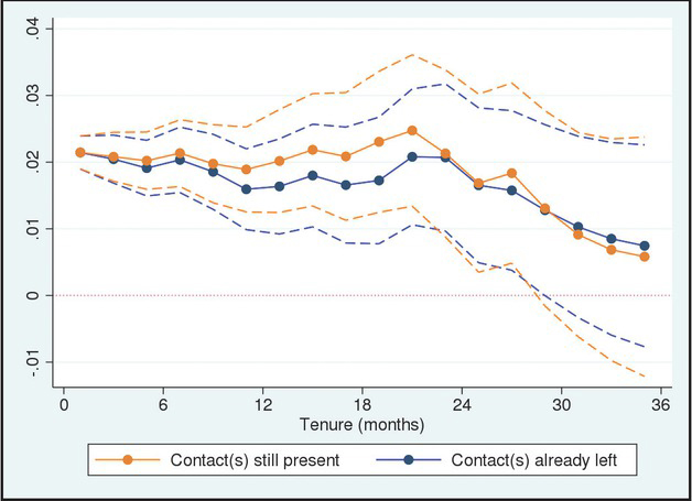
Figure 1
Wage-tenure profiles and referrer presence.
Note: The figure displays point estimations and 95% confidence intervals for two sets of estimations. The first set uses the proxy for contact presence upon entry, while in the other one the same indicator is set to zero if the original contact(s) left the firm by the given month. Both graphs present the parameter of eighteen separate regressions on the logarithm of daily earnings of male workers in the given month, for all odd months of the first three year of the employment spells. Female workers are included in the estimations, with a constant gender difference being assumed. Controlling for fixed effects is achieved by including pre-estimated individual and firm effects from the entry month equation. Additional controls are the same as listed in Table 3. Standard errors used for the confidence intervals are clustered at both firm level and individual level.
Table 8
Gains from links, second links, and similar workers
| Linked | 0.0484*** (0.0056) | 0.0194*** (0.0055) | 0.0188*** (0.0038) | 0.0102* (0.0042) | 0.0152*** (0.0035) | 0.0141** (0.0052) | 0.0036 (0.0023) | −0.0039 (0.0035) |
| Similar | 0.0131** (0.0050) | 0.0072 (0.0050) | 0.0150*** (0.0035) | −0.0091* (0.0041) | 0.0194*** (0.0032) | 0.0013 (0.0047) | −0.0044* (0.0023) | −0.0104** (0.0034) |
| Second | 0.0489** (0.0157) | 0.0125 (0.0173) | 0.0062 (0.0104) | 0.0302** (0.0111) | −0.0074 (0.0098) | 0.0238 (0.0142) | 0.0136* (0.0056) | 0.0064 (0.0091) |
| N | 938,791 | 479,919 | 938,791 | 938,791 | 917,835 | 550,362 | 938,791 | 938,791 |
| Ni | 603,975 | 189,756 | 603,975 | 603,975 | 603,955 | 215,546 | 603,975 | 603,975 |
| Nj | 105,061 | 60,367 | 105,061 | 105,061 | 84,105 | 105,022 | 105,061 | 105,061 |
| R2 | 0.326 | 0.860 | 0.199 | 0.198 | 0.452 | 0.611 | 0.050 | 0.088 |
[i] Note: Estimation results from the main regression on the logarithm of daily earnings upon job entry (Eq. (7)), without any and with two-way fixed effects, and the consecutive decomposition regressions on estimated firm and individual effects (Eqs (8-13)), respectively. The selection parameters in the columns reflect overall, within unit and between unit differences in individual and firm effects, respectively. Our parameters of interest are estimated with distinct indicators for the presence of former co-worker links, workers with similar working histories (those who share a common, former workplace with applicants), and second links (the former peers of the job-entrants’ former co-workers who did not fall into the similar working history group). The indicators marked in the table as Linked, Similar and Second respectively and were interacted with gender. Results for male workers are presented. For the list of additional controls, see Table 3. Standard errors are in parentheses and clustered at both firm level and individual level.
*Statistically significant at 0.05 level; **at 0.01 level; ***at 0.001 level.
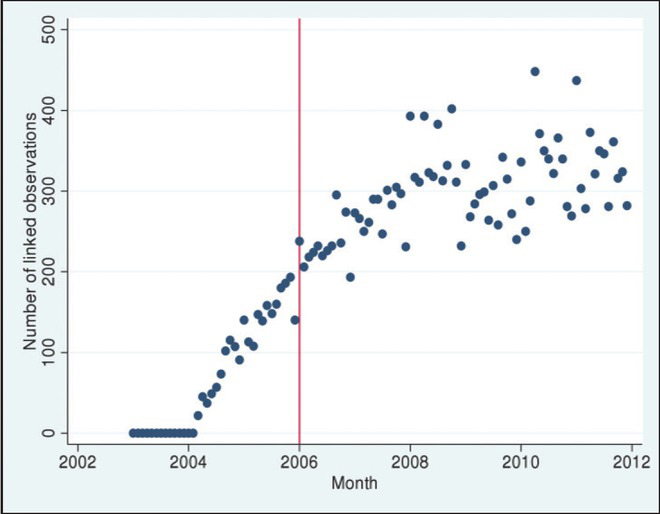
Figure A1
Number of linked workers over time.
Note: The figure displays the number of hires with co-worker links present in each calendar month from 2003 until 2011. The subsample used for the estimation is the same as in Table 2.
Table A1
Decomposition of co-worker gains by occupations - female results
| Manager | −0.0415 (0.0416) | −0.0809 (0.0463) | 0.0168 (0.0345) | 0.0226 (0.0216) | 0.0372 (0.0320) | 0.0804** (0.0289) | −0.0204 (0.0141) | −0.0579** (0.0198) |
| SkilledW | 0.1648*** (0.0425) | 0.0784 (0.0403) | 0.0157 (0.0293) | 0.0706** (0.0253) | 0.0015 (0.0264) | 0.0208 (0.0352) | 0.0142 (0.0152) | 0.0498* (0.0227) |
| UnskilledW | 0.0503** (0.0158) | 0.0081 (0.0194) | 0.0296* (0.0128) | 0.0126 (0.0113) | 0.0357** (0.0115) | 0.0150 (0.0157) | −0.0061 (0.0074) | −0.0024 (0.0098) |
| SkilledB | 0.0275* (0.0111) | −0.0107 (0.0140) | 0.0343*** (0.0090) | 0.0039 (0.0100) | 0.0298*** (0.0074) | 0.0170 (0.0124) | 0.0044 (0.0062) | −0.0132 (0.0089) |
| UnskilledB | −0.0097 (0.0140) | −0.0116 (0.0190) | 0.0158 (0.0102) | −0.0138 (0.0125) | 0.0178* (0.0090) | −0.0115 (0.0158) | −0.0020 (0.0057) | −0.0023 (0.0109) |
| N | 964,807 | 501,200 | 964,807 | 964,807 | 943,643 | 571,443 | 964,807 | 964,807 |
| Ni | 616,386 | 197,435 | 616,386 | 616,386 | 616,365 | 223,021 | 616,386 | 616,386 |
| Nj | 105,818 | 61,121 | 105,818 | 105,818 | 84,655 | 105,778 | 105,818 | 105,818 |
| R2 | 0.327 | 0.860 | 0.190 | 0.200 | 0.443 | 0.612 | 0.052 | 0.086 |
[i] Note: Estimation results from the main regression on the logarithm of daily earnings upon job entry (Eq. (7)), without any and with two-way fixed effects, and the consecutive decomposition regressions on estimated firm and individual effects (Eqs (8-13)), respectively. The selection parameters in the columns reflect overall, within unit and between unit differences in individual and firm effects, respectively. Our variable of interest, the proxy for links, is interacted with ten categories based on gender and five occupational categories: managers, skilled white-collar, unskilled white-collar, skilled blue-collar, and unskilled blue-collar workers. Only the parameters for female workers are presented. For the list of additional controls, see Table 3. Standard errors are in parentheses and clustered at both firm level and individual level.
*Statistically significant at the 0.05 level; **at the 0.01 level; ***at the 0.001 level.
Table A2
Decomposition of co-worker gains by occupations
| Manager | −0.0849*** (0.0223) | −0.0262 (0.0259) | −0.0508** (0.0183) | −0.0080 (0.0121) | −0.0397* (0.0171) | 0.0378 (0.0196) | −0.0111 (0.0079) | −0.0458*** (0.0109) |
| SkilledW | 0.1146*** (0.0240) | 0.0620** (0.0202) | 0.0046 (0.0158) | 0.0480** (0.0156) | −0.0026 (0.0141) | 0.0130 (0.0205) | 0.0072 (0.0088) | 0.0349* (0.0136) |
| UnskilledW | 0.0558*** (0.0126) | 0.0244 (0.0137) | 0.0223* (0.0096) | 0.0091 (0.0089) | 0.0249** (0.0086) | 0.0022 (0.0116) | −0.0026 (0.0056) | 0.0069 (0.0076) |
| SkilledB UnskilledB | 0.0507*** (0.0060) 0.0349*** (0.0072) | 0.0159* (0.0068) 0.0079 (0.0070) | 0.0236*** (0.0044) 0.0287*** (0.0044) | 0.0112* (0.0049) −0.0017 (0.0063) | 0.0156*** (0.0038) 0.0278*** (0.0041) | 0.0132* (0.0058) 0.0117 (0.0076) | 0.0079** (0.0030) 0.0009 (0.0028) | −0.0020 (0.0043) −0.0134** (0.0051) |
| N | 964,807 | 501,200 | 964,807 | 964,807 | 943,643 | 571,443 | 964,807 | 964,807 |
| Ni | 616,386 | 197,435 | 616,386 | 616,386 | 616,365 | 223,022 | 616,386 | 616,386 |
| Nj | 105,819 | 61,121 | 105,819 | 105,819 | 84,655 | 105,779 | 105,819 | 105,819 |
| R2 | 0.327 | 0.860 | 0.204 | 0.200 | 0.453 | 0.612 | 0.052 | 0.087 |
[i] Note: Estimation results from the main regression on the logarithm of daily earnings upon job entry (Eq. (7)), without any and with two-way fixed effects, and the consecutive decomposition regressions on estimated firm and individual effects (Eqs (8-13)), respectively. The selection parameters in the columns reflect overall, within unit and between unit differences in individual and firm effects, respectively. Our variable of interest, the proxy for links, is interacted with five occupational categories: managers, skilled white-collar, unskilled white-collar, skilled blue-collar, and unskilled blue-collar workers. For the list of additional controls, see Table 3. Standard errors are in parentheses and clustered at both firm level and individual level.
*Statistically significant at the 0.05 level; **at the 0.01 level; ***at the 0.001 level.
Table A3
Co-worker gains and skill requirements
| Linked | Skill | Interaction | |
|---|---|---|---|
| Baseline | 0.0172*** (0.0046) | − | − |
| Manual Dexterity | 0.0172*** (0.0047) | −0.0449*** (0.0020) | −0.0026 (0.0052) |
| Stamina | 0.0172*** (0.0047) | −0.0445*** (0.0019) | −0.0066 (0.0055) |
| Persistence | 0.0167*** (0.0046) | 0.0441*** (0.0014) | 0.0037 (0.0052) |
| Stress Tolerance | 0.0174*** (0.0046) | 0.0308*** (0.0014) | −0.0024 (0.0050) |
| Analytical Thinking | 0.0164*** (0.0046) | 0.0469*** (0.0015) | 0.0053 (0.0050) |
| Complex Problem Solving | 0.0159*** (0.0046) | 0.0546*** (0.0016) | 0.0056 (0.0048) |
| Active Learning | 0.0167*** (0.0046) | 0.0528*** (0.0015) | 0.0016 (0.0052) |
| Coordination | 0.0174*** (0.0046) | 0.0398*** (0.0014) | −0.0025 (0.0044 |
| Cooperation | 0.0171*** (0.0046) | 0.0203*** (0.0015) | −0.0022 (0.0052) |
| Adaptability/Flexibility | 0.0170*** (0.0046) | 0.0329*** (0.0015) | 0.0026 (0.0050) |
| Originality | 0.0163*** (0.0046) | 0.0436*** (0.0015) | 0.0066 (0.0052) |
| Innovation | 0.0158*** (0.0046) | 0.0329*** (0.0014) | 0.0081 (0.0048) |
| Independence | 0.0172*** (0.0046) | 0.0152*** (0.0015) | 0.0020 (0.0049) |
[i] Note: Estimation results from the main regression on the logarithm of daily earnings upon job entry with two-way fixed effects (Eq. (7)). Our variable of interest, the proxy for links, is interacted with the demeaned values of skill requirement measures from the O*Net database. For the list of additional controls, see Table 3. Standard errors are in parentheses and clustered at both firm level and individual level. All regressions are based on 483 418 observations and have an R2 between 0.860 and 0.861.
*Statistically significant at the 0.05 level; **at the 0.01 level; ***at the 0.001 level.