
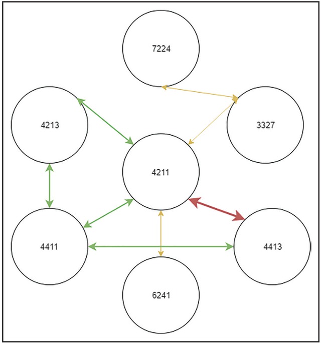
Figure 1
Creation of clusters of industries or labor markets.
Notes: The red link indicates that the two industries have more relative flows than any other pair (top pair). Green links indicate a strong relationship (the top three pairs or more than 90th of relative flows between industries); the sum of red and green links defines the preferred classification. Yellow links are weak connections, and the sum of yellow, green, and red links defines the flexible method.
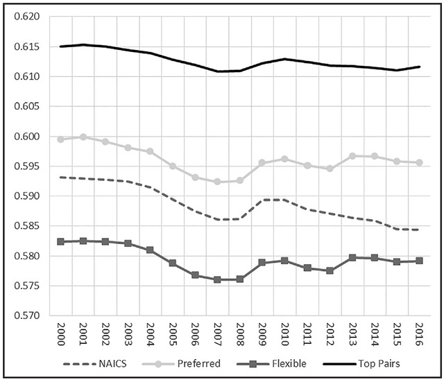
Figure 2
Evolution of the HHI in the United States: 2000–2016.
Note: The HHI is estimated by averaging industries and counties by year (weighted by population).
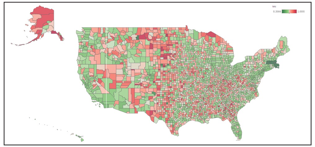
Figure 3
HHI in the United States across counties: 2000–2016.
Notes: The HHI is estimated by averaging industries and year by county (weighted by population). I use the hybrid method for the estimation of the HHI.
Table 1
Average number of establishments by HHI
| HHI | Low mobility | |||
|---|---|---|---|---|
| Mean | Median | Mean | Median | |
| Monopsony = 1 | 5.38 | 3.18 | 581.35 | 361.81 |
| 90th | 10.96 | 7.75 | 847.61 | 564.40 |
| 10th | 1,815.18 | 611.20 | 2,135.22 | 826.06 |
| 5th | 2,261.91 | 708.59 | 1,689.81 | 708.81 |
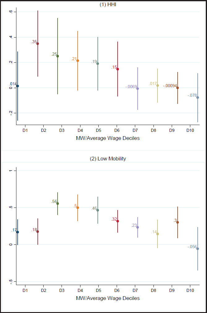
Figure 4
Effect of the minimum wage under monopsony by deciles.
Notes: I calculate MW/average wage and split the estimation in deciles. The higher the decile, the more binding is the minimum wage. All the estimations are evaluated with HHI or mobility equal to 1. HHI = 1 indicates full concentration. Mobility = 1 implies that the worker remains in the same industry for all the periods.
Table 2
Effects of the HHI and low mobility on the log of teenage wages
| (1) | (2) | |
|---|---|---|
| Dependent variable: Ln (wage) | HHI | Low mobility |
| HHI | −0.0993*** (0.0254) | |
| Low mobility | −0.127 (0.161) | |
| Constant | 8.128*** (0.716) | 6.784*** (1.391) |
| Observations | 199,168 | 18,121 |
| R-squared | 0.718 | 0.888 |
Robust clustered standard errors in parentheses by states.
**p < 0.05, *p < 0.1.
Notes: All specifications include two-way fixed effects (county and time). Control variables are the log of the total population, the log of teenage population, and log of total private-sector employment. HHI measures concentration: HHI = 0 implies perfect competition, and HHI = 1 means full concentration. Column (1) defines the labor market as clusters of industries, which consists of keeping only connections or links between industries with more relative flows of workers (top three links with highest flows with more than 90th percentile of relative flows between industries). Column (2) uses low mobility, which measures the percentage of workers who, when they change jobs, do not change industries. See Section 4 for more details.
Table 3
Effects of the log of the MW interacted with the HHI and low mobility on the log of teenage employment
| (1) | (2) | |
|---|---|---|
| Dependent variable: Ln (teen employment) | HHI | Low mobility |
| Monopsony variable (HHI or LM) | −0.833** (0.324) | −0.915*** (0.235) |
| Monopsony × Ln (MW) | 0.459** (0.180) | 0.476*** (0.124) |
| Elasticity of the MW depending on monopsony | ||
| Monopsony = 0 | −0.418*** (0.112) | −0.183 (0.146) |
| Monopsony = 0.2 | −0.326*** (0.0931) | −0.0876 (0.148) |
| Monopsony = 0.4 | −0.234*** (0.0858) | 0.00755 (0.155) |
| Monopsony = 0.6 | −0.142 (0.0930) | 0.103 (0.165) |
| Monopsony = 0.8 | −0.0507 (0.112) | 0.198 (0.179) |
| Monopsony = 1 | 0.0411 (0.138) | 0.293 (0.194) |
| Constant | −0.193 (0.741) | −1.786 (1.553) |
| Observations | 199,231 | 18,126 |
| R-squared | 0.988 | 0.989 |
Robust clustered standard errors in parentheses by states.
*p < 0.1.
Notes: All specifications include two-way fixed effects (county and time). Control variables are log of the total population, the log of teenage population, and log of total private-sector employment. HHI measures concentration: HHI = 0 implies perfect competition, and HHI = 1 means full concentration. Column (1) defines the labor market as clusters of industries, which consists of keeping only connections or links between industries with more flows of workers (top three links with highest flows with more than 90th percentile of relative flows between industries). Column (2) uses low mobility, which measures the percentage of workers who, when they change jobs, do not change industries. See Section 4 for more details.
Table 4
Percentage of the teenage employment by the significance of the minimum wage effects depending on the monopsony variable
| Share of the total teenage employment (%) | |
|---|---|
| Negative significant | 55.81 |
| Negative | 44.06 |
| Positive | 0.12 |
| Positive significant | 0.00 |
[i] Notes: I am using the “hybrid” classification, but the results are very similar to the other classifications. The calculations are computed as follows: (1) I estimate the coefficients with the regression models, (2) use the coefficients to estimate the MW effects on the teenage employment, (3) determine at what level of HHI the MW effect is negative, negative significant, positive, and positive significant, (4) aggregate the employment by HHI, and (5) calculate the shares of employment where the MW has negative, negative significant, positive, positive significant effects. The estimation is based on the coefficient of the regression model of column (1) in Table 4.
Table 5
Robustness check: effects of the log of the MW interacted with all the classifications of clusters for the HHI on the log of teenage employment
| (1) | (2) | (3) | |
|---|---|---|---|
| Dependent variable: Ln (teen employment) | NAICS | Flexible | Top pairs |
| Monopsony variable (HHI or LM) | −0.972*** (0.341) | −0.920*** (0.336) | −0.998** (0.377) |
| Monopsony × Ln (MW) | 0.527*** (0.189) | 0.504** (0.191) | 0.523** (0.204) |
| Elasticity of the MW depending on monopsony | |||
| Monopsony = 0 | −0.458*** (0.133) | −0.438*** (0.125) | −0.461*** (0.145) |
| Monopsony = 0.2 | −0.353*** (0.109) | −0.338*** (0.102) | −0.357*** (0.117) |
| Monopsony = 0.4 | −0.247*** (0.0958) | −0.237*** (0.0912) | −0.252** (0.0990) |
| Monopsony = 0.6 | −0.142 (0.0961) | −0.136 (0.0952) | −0.147 (0.0959) |
| Monopsony = 0.8 | −0.0365 (0.110) | −0.0354 (0.113) | −0.0427 (0.109) |
| Monopsony = 1 | 0.0690 (0.134) | 0.0653 (0.139) | 0.0619 (0.134) |
| Constant | −0.119 (0.708) | −0.140 (0.711) | −0.0320 (0.717) |
| Observations | 199,231 | 199,231 | 199,231 |
| R-squared | 0.988 | 0.988 | 0.988 |
Robust clustered standard errors in parentheses by states.
* p < 0.1.
Notes: All specifications include two-way fixed effects (county and time). Control variables are the log of the total population, log of teenage population, and log of total private-sector employment. HHI measures concentration: HHI = 0 implies perfect competition, and HHI = 1 means full concentration. Column (1) defines the labor market by three-digit NAICS code. In column (2), the cluster is defined by all the links; for instance, if industry A is connected to industry B, and industry B is connected to industry C, then A and C are connected. Column (3) only considers as a cluster the pair of industries with more relative flows between each other. See Appendix B for more details.
Table 6
Effects of the log of the MW interacted with the HHI and low mobility on the log of teenage employment, allowing different effects of MW by industry
| (1) | (2) | (3) | (4) | (5) | |
|---|---|---|---|---|---|
| Dependent variable: Ln (teen employment) | HHI | Low mobility | NAICS | Flexible | Top pairs |
| Ln (MW) | −0.233 (0.130) | 0.0907 (0.261) | −0.160 (0.129) | −0.190 (0.133) | −0.142 (0.140) |
| HHI or low mobility | −0.714*** (0.120) | −0.119* (0.0691) − | 0.585*** (0.117) | −0.712*** (0.126) | −0.335*** (0.121) |
| HHI or low mobility × Ln (MW) | 0.389*** (0.0615) | 0.0685* (0.0357) | 0.314*** (0.0602) | 0.365*** (0.0625) | 0.257*** (0.0654) |
| Constant | −0.496 (0.333) | −7.681** (3.136) | 0.384 (0.371) | 1.147*** (0.350) | −1.400*** (0.370) |
| Observations | 2,201,021 | 18,001 | 1,954,252 | 1,921,138 | 2,603,089 |
| R-squared | 0.818 | 0.970 | 0.831 | 0.831 | 0.793 |
Robust clustered standard errors in parentheses by states.
Notes: All specifications include three-way fixed effects (county, time, and industry). Control variables are the log of the total population, log of teenage population, and log of total private-sector employment. HHI measures concentration: HHI = 0 implies perfect competition, and HHI = 1 means full concentration. In addition, all the specifications include interactions of Ln (MW) by industry. The coefficient reported for Ln (MW) is the effect evaluated in the average of each industry for HHI = 0. Column (1) defines the labor market as clusters of industries, which consists of keeping only connections or links between industries with more relative flows of workers (top three links with highest flows with more than 90th percentile of relative flows between industries). Column (2) uses low mobility, which measures the percentage of workers who, when they change jobs, do not change industries. Column (3) defines the labor market by three-digit NAICS code. In column (4), the cluster is defined by all the links; for instance, if industry A is connected to industry B, and industry B is connected to industry C, then A and C are connected. Column (5) only considers as a cluster the pair of industries with more relative flows between each other. See Section 4 for more details.
Table 7
Effects of the log of the MW interacted with the HHI and low mobility on the log of teenage employment, average of the HHI in different periods
| (1) | (2) | |
|---|---|---|
| Dependent Variable: Ln (Emp) | HHI | Low mobility |
| Panel A: Using the period average | ||
| Ln (MW) | −0.501*** (0.142) | −1.123*** (0.192) |
| HHI or Mobility (average) × Ln (MW) | 0.575** (0.238) | 1.905*** (0.376) |
| Constant | −0.846 (0.780) | −2.918** (1.098) |
| Observations | 200,052 | 26,657 |
| R-squared | 0.988 | 0.988 |
| Panel B: Using the average from 2000 to 2001 | ||
| Ln (MW) | −0.306** (0.131) | −0.999*** (0.294) |
| HHI or mobility (average) × Ln (MW) | 0.330 (0.200) | 1.711*** (0.514) |
| Constant | −0.967 (0.930) | −2.906 (1.896) |
| Observations | 168,219 | 14,036 |
| R-squared | 0.988 | 0.988 |
Robust clustered standard errors in parentheses by states.
*p < 0.1.
Notes: All specifications include two-way fixed effects (county and time). Control variables are the log of the total population, log of teenage population, and total private-sector employment. HHI measures concentration: HHI = 0 implies perfect competition, and HHI = 1 means full concentration. Column (1) defines the labor market as clusters of industries, which consists of keeping only connections or links between industries with more relative flows of workers (top three links with highest flows with more than 90th percentile of relative flows between industries). Column (2) uses low mobility, which measures the percentage of workers who, when they change jobs, do not change industries. See Section 4 for more details. The HHI and mobility do not vary over time; thus, the coefficients are dropped due to collinearity with time. Panel A uses HHI average of all the period (2000–2016) and Panel B uses the average from 2000 to 2001.
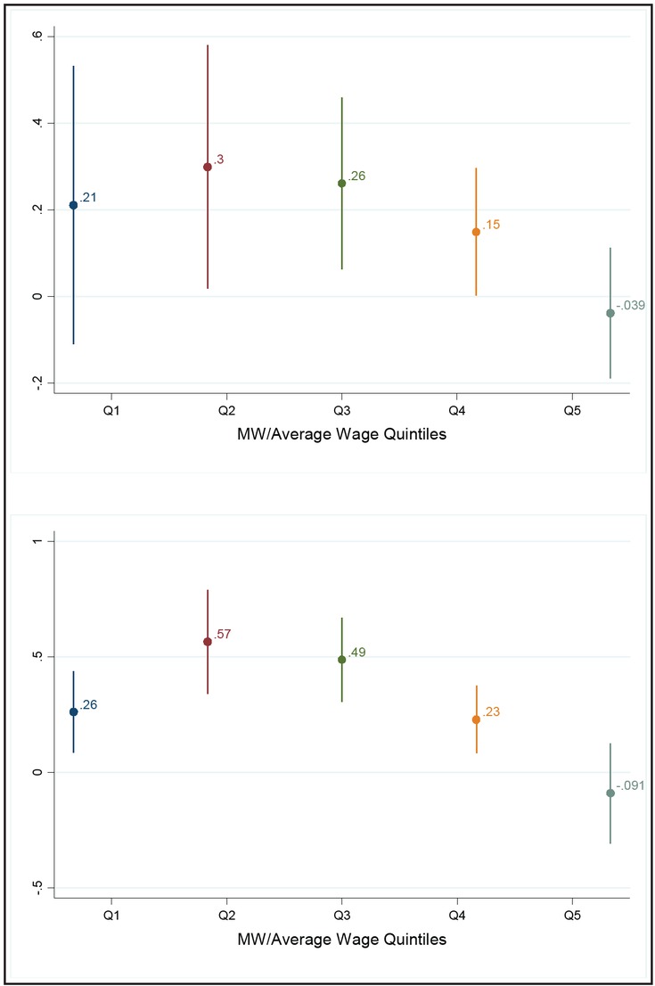
Figure A1
Effect of the minimum wage under monopsony by quintiles.
Notes: I calculate MW/average wage and split the estimation in quintiles. The higher the quintile, the more binding the minimum wage is. All the estimations are evaluated with HHI or mobility equal to 1. HHI = 1 indicates full concentration. Mobility = 1 implies that the worker remains in the same industry for all the periods.
Table A1
Statistics of the HHI and low mobility by method of estimation
| Mean | Median | Min | Max | SD | |
|---|---|---|---|---|---|
| HHI | 0.595 | 0.575 | 0.077 | 1.000 | 0.070 |
| Low mobility | 0.608 | 0.608 | 0.000 | 1.000 | 0.071 |
| NAICS | 0.587 | 0.570 | 0.169 | 1.000 | 0.069 |
| Flexible | 0.578 | 0.560 | 0.125 | 1.000 | 0.069 |
| Top pairs | 0.612 | 0.598 | 0.331 | 1.000 | 0.060 |
Table A2
Effects of the log of the minimum wage on HHI and low mobility
| (1) | (2) | (3) | (4) | (5) | |
|---|---|---|---|---|---|
| Dependent variable: HHI or low mobility | Hybrid | Low mobility | NAICS | Flexible | Top pairs |
| Ln (MW) | −0.00382 (0.00514) | −0.00325 (0.0165) | 0.00301 (0.00510) | −0.00729 (0.00636) | −0.00347 (0.00307) |
| Constant | 1.083*** (0.0914) | 1.174*** (0.419) | 1.123*** (0.0666) | 1.090*** (0.125) | 1.082*** (0.0681) |
| Observations | 199,421 | 18,126 | 199,421 | 199,421 | 199,421 |
| R-squared | 0.909 | 0.365 | 0.974 | 0.856 | 0.981 |
Robust clustered standard errors in parentheses by states.
**p < 0.05, *p < 0.1.
Notes: All specifications include two-way fixed effects (county and time). Control variables are the log of the total population, log of teenage population, and log of total private-sector employment. Column (1) defines the labor market as clusters of industries, which consists of keeping only connections or links between industries with more relative flows of workers (top three links with highest flows with more than 90th percentile of relative flows between industries). Column (2) uses low mobility, which measures the percentage of workers who, when they change jobs, do not change industries. Column (3) defines the labor market by three-digit NAICS code. In column (4), the cluster is defined by all the links; for instance, if industry A is connected to industry B, and industry B is connected to industry C, then A and C are connected. Column (5) only considers as a cluster the pair of industries with more relative flows between each other. See Section 4 for more details.
Table A3
Effects of the log of the MW interacted with the HHI and low mobility on the log of teenage employment (HHI calculated only for teenage workers)
| (1) | (2) | (3) | (4) | (5) | |
|---|---|---|---|---|---|
| Dependent variable: Ln (teen employment) | Hybrid | Low mobility | NAICS | All nodes | Top pairs |
| Ln (MW) | −0.223** (0.0938) | −0.167 (0.138) | −0.188* (0.0944) | −0.165* (0.0928) | −0.543*** (0.124) |
| Monopsony variable (HHI or LM) | −0.381*** (0.138) − | 0.859*** (0.242) | −0.241** (0.106) | −0.349 (0.228) | −1.173*** (0.342) |
| Monopsony × Ln (MW) | 0.223*** (0.0757) | 0.447*** (0.127) | 0.126** (0.0558) | 0.196 (0.122) | 0.631*** (0.184) |
| Constant | −0.494 (0.723) | −1.806 (1.539) | −0.416 (0.750) | −0.577 (0.740) | −0.0139 (0.727) |
| Observations | 195,205 | 18,121 | 195,205 | 195,205 | 199,123 |
| R-squared | 0.988 | 0.989 | 0.988 | 0.988 | 0.988 |
Robust clustered standard errors in parentheses by states.
Notes: All specifications include two-way fixed effects (county and time). Control variables are the log of the total population, log of teenage population, and log of total private-sector employment. HHI measures concentration: HHI = 0 implies perfect competition, and HHI=1 implies full concentration. Column (1) defines the labor market as clusters of industries, which consists of keeping only connections or links between industries with more relative flows of workers (top three links with highest flows with more than 90th percentile of relative flows between industries). Column (2) uses low mobility, which measures the percentage of workers who, when they change jobs, do not change industries. Column (3) defines the labor market by three-digit NAICS code. In column (4), the cluster is defined by all the links; for instance, if industry A is connected to industry B, and industry B is connected to industry C, then A and C are connected. Column (5) only considers as a cluster the pair of industries with more relative flows between each other. See Section 4 for more details.
Table A4
Effects of the log of the MW interacted with the low mobility on the log of teenage employment (low mobility using workers who moved to other county)
| (1) | |
|---|---|
| Dependent variable: Ln (teen employment) | Low mobility |
| Monopsony variable (HHI or LM) | −0.968*** (0.275) |
| Monopsony × Ln (MW) | 0.503*** (0.145) |
| Elasticity of the MW depending on monopsony | |
| Monopsony = 0 | −0.184 (0.158) |
| Monopsony = 0.2 | −0.0843 (0.161) |
| Monopsony = 0.4 | 0.0158 (0.169) |
| Monopsony = 0.6 | 0.116 (0.181) |
| Monopsony = 0.8 | 0.216 (0.197) |
| Monopsony = 1 | 0.316 (0.215) |
| Constant | −1.691 (1.761) |
| Observations | 18,127 |
| R-squared | 0.988 |
Robust clustered standard errors in parentheses by states.
**p < 0.05, *p < 0.1.
Notes: All specifications include two-way fixed effects (county and time). Control variables are the log of the total population, log of teenage population, and log of total private-sector employment. HHI measures concentration: HHI = 0 implies perfect competition, and HHI = 1 means full concentration. Low mobility, which measures the percentage of workers who, when they change jobs, do not change industries, includes workers who moved to other counties.
Table A5
Effects of the log of the MW interacted with the HHI and low mobility on the log of prime age
| (1) | (2) | (3) | (4) | (5) | |
|---|---|---|---|---|---|
| Dependent variable: Ln (prime age employment) | HHI | Low mobility | NAICS | Flexible | Top pairs |
| Ln (MW) | −0.0272 (0.0866) | 0.139 (0.113) | 0.0345 (0.0797) − | 0.00485 (0.0830) | 0.0400 (0.0992) |
| HHI | 0.149 (0.296) | 0.317 (0.286) | 0.199 (0.290) | 0.389 (0.322) | |
| HHI × Ln (MW) | 0.0514 (0.151) | −0.0572 (0.141) | 0.0136 (0.148) | −0.0601 (0.160) | |
| Low mobility | 0.452 (0.368) | ||||
| Low mobility × Ln (MW) | −0.220 (0.186) | ||||
| Constant | 0.960 (0.672) | 2.732*** (0.602) | 0.897 (0.678) | 0.930 (0.683) | 0.828 (0.665) |
| Observations | 204,984 | 18,130 | 204,984 | 204,984 | 204,984 |
| R-squared | 0.999 | 0.999 | 0.999 | 0.999 | 0.999 |
Robust clustered standard errors in parentheses by states.
**p < 0.05, *p < 0.1.
Notes: All specifications include two-way fixed effects (county and time). Control variables are the log of the total population, log of prime-age population, and log of total private-sector employment. HHI measures concentration: HHI = 0 implies perfect competition, and HHI = 1 implies full concentration. Column (1) defines the labor market as clusters of industries, which consists of keeping only connections or links between industries with more relative flows of workers (top three links with highest flows with more than 90th percentile of relative flows between industries). Column (2) uses low mobility, which measures the percentage of workers who, when they change jobs, do not change industries. Column (3) defines the labor market by three-digit NAICS code. In column (4), the cluster is defined by all the links; for instance, if industry A is connected to industry B, and industry B is connected to industry C, then A and C are connected. Column (5) only considers as a cluster the pair of industries with more relative flows between each other. See Section 4 for more details.