
Table 1
Education Responsibilities and transfers by level of government
| Central government | |||
|---|---|---|---|
| Set school curriculum | Set teacher wages | Set general guidelines | Financial transfers to local authorities |
| Local authorities | |||
| Up to 2002 (Law 60/1993) | From 2002 onward (Law 715/2001) | ||
| Autonomous municipalities | |||
| Transfers: | 84% to department 16% to municipality | Transfers: | 100% to municipality |
| Teacher hiring, training and | Teacher hiring, training and | ||
| placement School infrastructure and materials School transport and any auxiliary program | Departments and municipalities, under departments’ supervision | placement School infrastructure and materials School transport and any auxiliary program | Municipality only |
| Nonautonomous municipalities | |||
| Transfers: | 97% to department 3% to municipality | ||
| Teacher hiring, training and placement School infrastructure and materials School transport and any auxiliary program | Department only (maintenance duties for municipality) | ||
[i] Notes: Author’s illustration, based on Laws 60/1993, 115/1994, and 715/2001 (Congreso, 1993, 1994, 2001); Borjas and Acosta (2000); and National Planning Department (Departamento Nacional de Planeación[DNP]; 2002). Percentages are author’s derivation: pre-reform values are based on 2001 data in DNP (2002, p.16); post-reform data are based on 2004 data in DNP (2004a, 2004b). Percentages for departments include the four special districts.
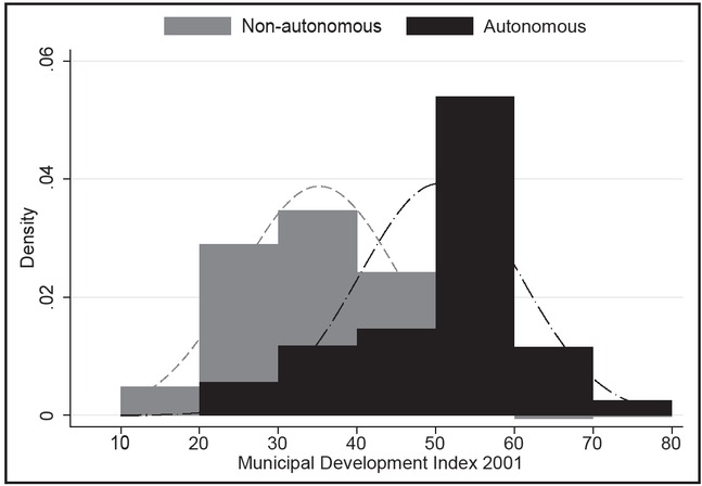
Figure 1
Municipal development in the empirical sample. Notes: The figure plots the MDI values for the year 2001 for our sample of cities, distinguishing between those that acquired autonomy in 2002 (darker) and those that did not (lighter). The two distributions overlap in transparency (darkest). Normal curves are overlaid.
Table 2
The effect of municipal autonomy on test scores
| Period average | Over-time evolution | ||||||
|---|---|---|---|---|---|---|---|
| (1) | (2) | (3) | (4) | (5) | (6) | (7) | |
| Naive | Baseline | 2002–2003 | 2004–2005 | 2006–2007 | 2008–2009 | 2010–2012 | |
| Autonomy | 0.67*** | −2.53*** | −0.67 | −1.17* | −1.47** | −2.73*** | −5.54*** |
| (0.21) | (0.87) | (0.62) | (0.67) | (0.70) | (1.00) | (1.44) | |
| Autonomy × MDI | 0.06*** | 0.02 | 0.03* | 0.04*** | 0.07*** | 0.14*** | |
| (0.02) | (0.01) | (0.01) | (0.01) | (0.02) | (0.03) | ||
| Municipality FE | Yes | Yes | Yes | Yes | Yes | Yes | Yes |
| Time dummies | Yes | Yes | Yes | Yes | Yes | Yes | Yes |
| N | 8,734 | 8,734 | 2,742 | 2,665 | 2,707 | 2,705 | 3,367 |
| N groups | 692 | 692 | 692 | 692 | 692 | 692 | 692 |
| R-sq. | 0.51 | 0.51 | 0.51 | 0.77 | 0.69 | 0.44 | 0.44 |
| Mean y | 42.34 | 42.34 | 41.33 | 41.54 | 42.69 | 41.89 | 42.41 |
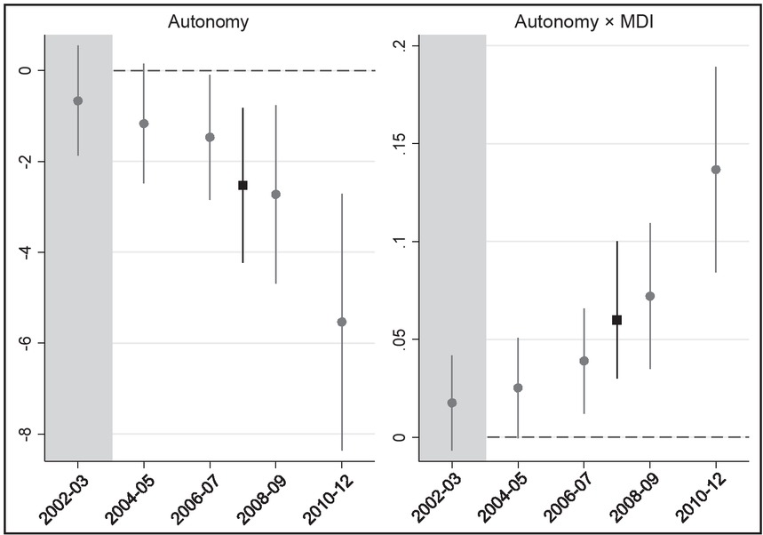
Figure 2
The effect of municipal autonomy on test scores. Notes: The figure plots the coefficients on municipal autonomy (left) and on the interaction between autonomy and development (right), estimated at different postreform periods with baseline model (2). Black squares indicate over-time average estimates, and spikes represent 95% confidence intervals. The reform transition period is shaded in gray.
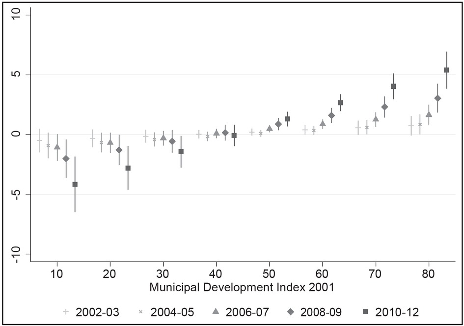
Figure 3
The overall effect of municipal autonomy on test scores, by MDI and time. Notes: The figure plots the marginal effects of municipal autonomy on test scores, by level of municipal development (on x-axis) and at different postreform periods (see different marker shapes). Spikes represent 95% confidence intervals.
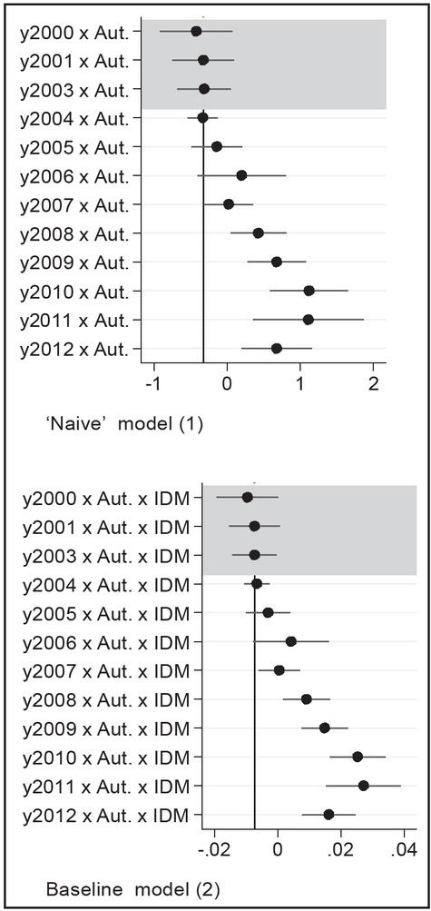
Figure 4
Leads and lags. Notes: The figure plots interactions between autonomy and year dummies (“naive model”) and three-way interactions between autonomy, local development, and year dummies (baseline model); point estimates represent differences with respect to 2002. Spikes represent 95% confidence intervals. Pre-reform and transition years are shaded in gray.
Table 3
Leads and lags
| (1) | (2) | |
|---|---|---|
| Naive | Baseline | |
| y2000 × Aut. (× MDI) | −0.42* (0.25) | −0.01* (0.00) |
| y2001 × Aut. (× MDI) | −0.33 (0.22) | −0.01* (0.00) |
| y2003 × Aut. (× MDI) | −0.31* (0.19) | −0.01** (0.00) |
| y2004 × Aut. (× MDI) | −0.33*** (0.10) | −0.01*** (0.00) |
| y2005 × Aut. (× MDI) | −0.14 (0.18) | 0.00 (0.00) |
| y2006 × Aut. (× MDI) | 0.20 (0.31) | 0.00 (0.01) |
| y2007 × Aut. (× MDI) | 0.02 (0.17) | 0.00 (0.00) |
| y2008 × Aut. (× MDI) | 0.43** (0.19) | 0.01** (0.00) |
| y2009 × Aut. (× MDI) | 0.68*** (0.20) | 0.01*** (0.00) |
| y2010 × Aut. (× MDI) | 1.12*** (0.27) | 0.03*** (0.00) |
| y2011 × Aut. (× MDI) | 1.11*** (0.38) | 0.03*** (0.01) |
| y2012 × Aut. (× MDI) | 0.68*** (0.25) | 0.02*** (0.00) |
| Municipality FE | Yes | Yes |
| Time dummies | Yes | Yes |
| N | 8,734 | 8,734 |
| N groups | 692 | 692 |
| R-sq. | 0.51 | 0.51 |
| Mean y | 42.34 | 42.34 |
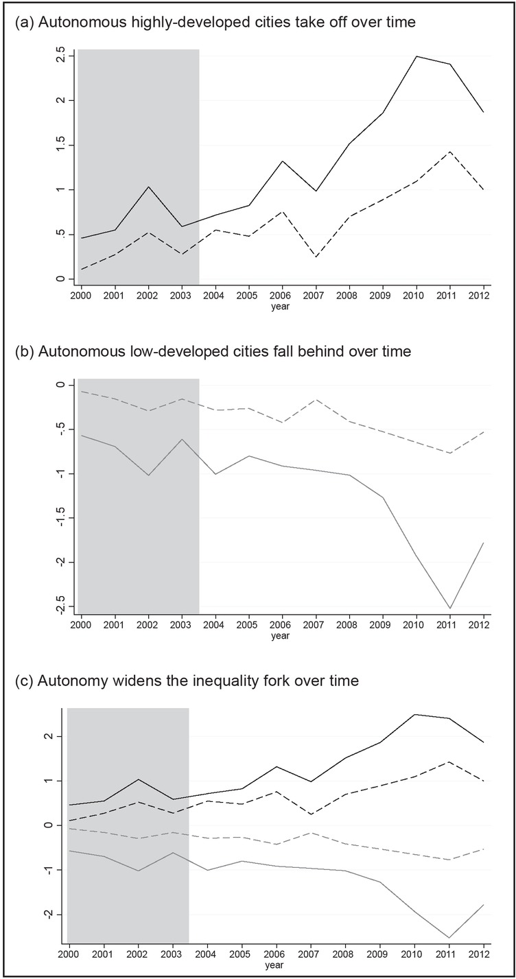
Figure 5
Evolution of test scores for the two groups of cities over time. (a) Autonomous highly developed cities take off over time. (b) Autonomous low-developed cities fall behind over time. (c) Autonomy widens the inequality fork over time. Notes: The figure shows the test score deviations from the national average. Autonomous cities are solid, and nonautonomous ones are dashed. Highly developed cities are in darker color, low-developed ones are in lighter color. Pre-reform and transition years are shaded in gray.
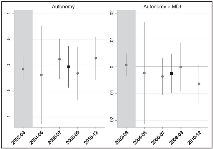
Figure 6
The effect of municipal autonomy on number of test takers (% change). Notes: The figure plots the coefficients on municipal autonomy (left) and on the interaction between autonomy and development (right), estimated at different postreform periods. Black squares indicate over-time average estimates, and spikes represent 95% confidence intervals.
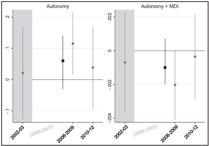
Figure 7
The effect of municipal autonomy on share of disadvantaged-background test takers. Notes: The figure plots the coefficients on municipal autonomy (left) and on the interaction between autonomy and development (right), estimated at different postreform periods. Black squares indicate over-time average estimates, and spikes represent 95% confidence intervals. In the period 2004–2007, socioeconomic status data were not collected.
Table 4
Education finance and administration quality in autonomous cities
| High-D | Low-D | Difference (%) | N | N cities | ||
|---|---|---|---|---|---|---|
| Education finance | ||||||
| Total spending | 1,175.24 (28.11) | 1,088.50 (61.19) | 86.74 (66.24) | (+8%) | 242 | 35 |
| Salaries | 939.99 (21.00) | 861.49 (45.35) | 78.50 (49.41) | (+9%) | ||
| Infrastructure and materials | 97.38 (6.44) | 109.75 (13.66) | −12.37 (15.10) | (−11%) | ||
| Others | 87.18 (6.77) | 70.21 (13.12) | 16.97 (15.65) | (+24%) | ||
| Student–teacher ratios | 27.33 (0.23) | 24.75 (0.36) | 2.58*** (0.51) | (+10%) | 145 | 35 |
| Transfers received | 1,147.48 (48.92) | 1,130.76 (25.60) | 16.72 (60.20) | (+2%) | 334 | 35 |
| Administrative indicators | ||||||
|---|---|---|---|---|---|---|
| Correctness standards | 79.30 (1.46) | 71.40 (4.93) | 7.90* (3.88) | (+11%) | 236 | 35 |
| Capacity | 72.46 (1.56) | 43.85 (4.20) | 28.61*** (3.89) | (+65%) | 236 | 35 |
| Corruption | 98.70 (6.03) | 109.58 (22.94) | −10.88 (28.26) | (−10%) | 89 | 32 |
Notes: Financial data are expressed in 2008 Colombian Pesos per pupil. Standard deviations of the means and standard errors of the difference within parentheses.
** p<0.05,
Table A1
Descriptive statistics
| All cities | Autonomous | Nonautonomous | |
|---|---|---|---|
| Test-related | |||
| Test scores (pre-reform) | 41.44 (1.52) | 41.74 (1.34) | 41.42 (1.53) |
| Test scores (postreform) | 42.51 (2.30) | 43.39 (2.35) | 42.46 (2.29) |
| Number of test takers | 296.16 (483.57) | 1,839.40 (1,116.16) | 213.70 (214.11) |
| Share of low-SES test takers | 0.88 (0.10) | 0.78 (0.11) | 0.87 (0.10) |
| Municipal characteristics | |||
| Municipal Development Index 2001 | 36.03 (10.81) | 50.67 (10.25) | 35.25 (10.27) |
| Population in 2002 (thousands) | 36,834.28 (52,225.38) | 221,149.10 (106,137.50) | 26,855.00 (18,259.58) |
| Education finance (postreform) | |||
|---|---|---|---|
| Total spending (per student) | - | 1,159.46 (398.03) | - |
| Salaries | - | 925.72 (297.42) | - |
| Infrastructure and materials | - | 99.63 (90.55) | - |
| Others | - | 84.09 (93.91) | - |
| Student–teacher ratio | - | 26.85 (2.59) | - |
| Transfers received (per student) | - | 1,144.58 (416.21) | - |
| Number of cities | 692 | 35 | 658 |
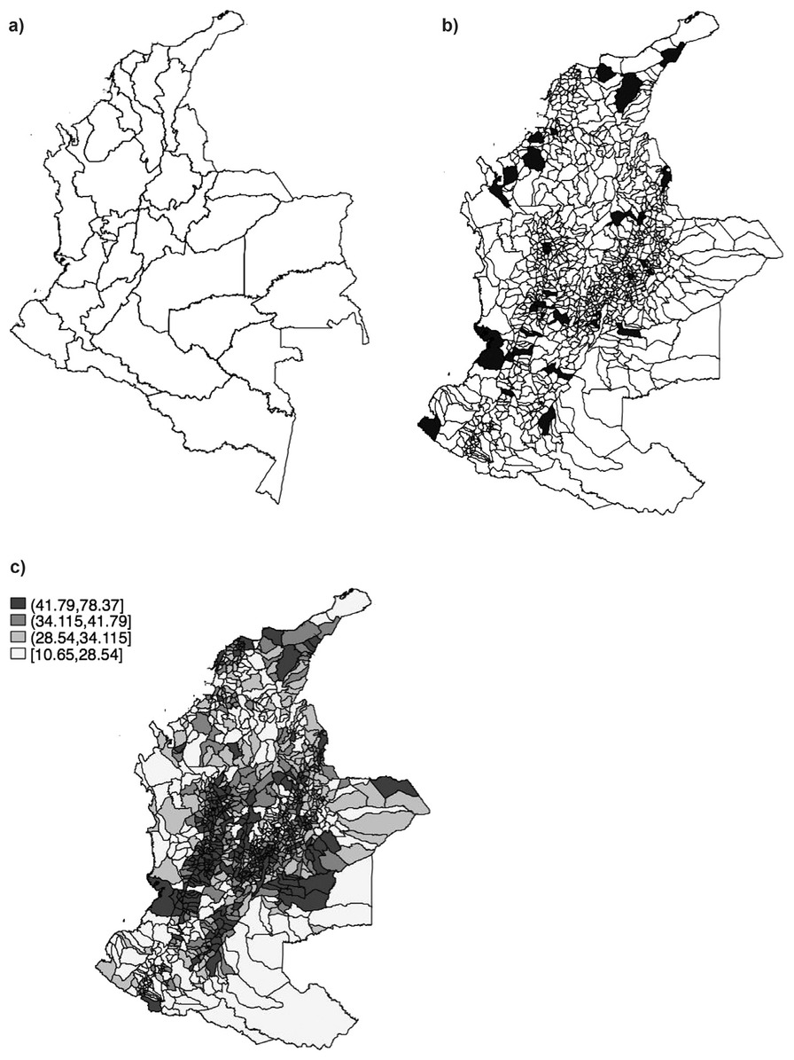
Figure A1
Maps of Colombia: a) Colombia’s departments; b) Colombia’s municipalities in black, those which were assigned autonomy over education in 2002; c) Distribution of Municipal Development Index in 2001. Note: In maps b) and c), the rural southeast is omitted to increase readability in the densely populated area.
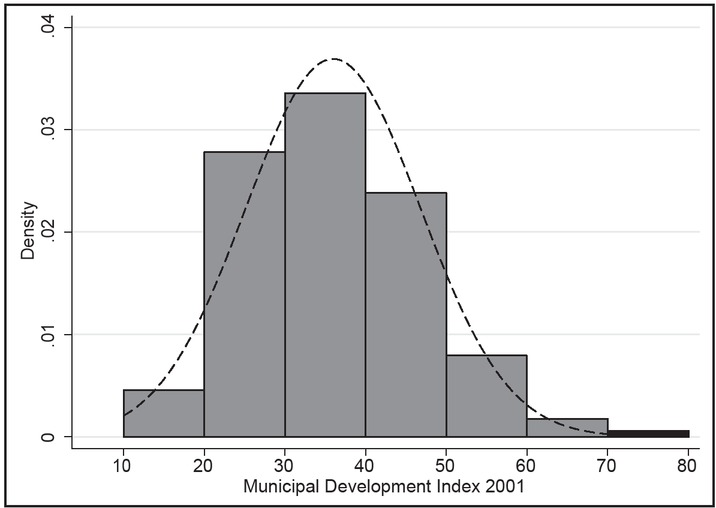
Figure A2
Municipal development index in the empirical sample. Notes: The figure plots the 2001 MDI values for our sample of cities. The normal curve is overlaid.
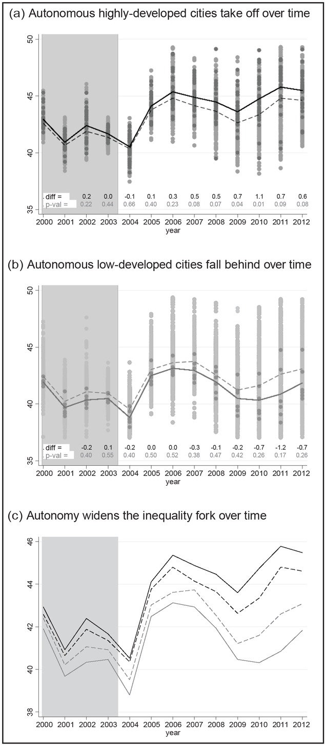
Figure A3
Evolution of test scores for the two groups of cities over time. Notes: The figure shows the evolution of test score averages over time. Autonomous cities are solid, nonautonomous ones are dashed; highly developed cities are darker, and low-developed ones are lighter. In subfigures (a) and (b) at the bottom, differences between the postreform gap and the pre-reform (2001) gap are indicated (H0: diff = 0). Pre-reform and transition years are shaded in gray.
Table A2
The effect of municipal autonomy on test scores – other subjects
| Subject | Period average | Over-time evolution | |||||
|---|---|---|---|---|---|---|---|
| (1) | (2) | (3) | (4) | (5) | (6) | (7) | |
| Naive | Baseline | 2002–2003 | 2004–2005 | 2006–2007 | 2008–2009 | 2010–2012 | |
| Critical reading | |||||||
| Autonomy | 0.28*** (0.11) | −0.56 (0.42) | −0.47* (0.27) | −0.01 (0.78) | 0.33 (0.75) | 0.10 (0.59) | −2.13*** (0.66) |
| Autonomy × MDI | 0.02** (0.01) | 0.01 (0.01) | 0.00 (0.01) | 0.00 (0.02) | 0.00 (0.01) | 0.06*** (0.01) | |
| Sciences | |||||||
| Autonomy | 0.21*** (0.08) | −0.58* (0.32) | −0.65 (0.52) | −0.13 (0.38) | −0.06 (0.41) | −0.08 (0.39) | −1.65*** (0.55) |
| Autonomy × MDI | 0.02** (0.01) | 0.02* (0.01) | 0.00 (0.01) | 0.00 (0.01) | 0.00 (0.01) | 0.04*** (0.01) | |
| Time dummies | Yes | Yes | Yes | Yes | Yes | Yes | Yes |
| N | 8,734 | 8,734 | 2,742 | 2,665 | 2,707 | 2,705 | 3,367 |
| N groups | 692 | 692 | 692 | 692 | 692 | 692 | 692 |
| R-sq. | 0.74 | 0.74 | 0.46 | 0.75 | 0.65 | 0.40 | 0.65 |
Table A3
The effect of municipal autonomy on number of test takers (% change)
| Period average | Over-time evolution | ||||||
|---|---|---|---|---|---|---|---|
| (1) | (2) | (3) | (4) | (5) | (6) | (7) | |
| naïve | Baseline | 2002–2003 | 2004–2005 | 2006–2007 | 2008–2009 | 2010–2012 | |
| Autonomy | −0.16*** (0.04) | −0.03 (0.20) | −0.08 (0.12) | −0.19 (0.48) | 0.11 (0.20) | −0.16 (0.26) | 0.13 (0.21) |
| Autonomy × MDI | 0.00 (0.00) | 0.00 (0.00) | 0.00 (0.01) | 0.00 (0.00) | 0.00 (0.00) | −0.01* (0.00) | |
| Municipality FE | Yes | Yes | Yes | Yes | Yes | Yes | Yes |
| Time dummies | Yes | Yes | Yes | Yes | Yes | Yes | Yes |
| N | 8,734 | 8,734 | 2,742 | 2,665 | 2,707 | 2,705 | 3,367 |
| N groups | 692 | 692 | 692 | 692 | 692 | 692 | 692 |
| R-sq. | 0.27 | 0.27 | 0.05 | 0.10 | 0.35 | 0.09 | 0.57 |
Table A4
The effect of municipal autonomy on share of low-SES test takers
| Period average | Over-time evolution | |||||
|---|---|---|---|---|---|---|
| (1) | (2) | (3) | (4) | (5) | (6) | |
| naïve | Baseline | 2002–2003 | (2004–2007) | 2008–2009 | 2010–2012 | |
| Autonomy | 0.01 (0.01) | 0.06 (0.04) | 0.02 (0.08) | 0.12** (0.05) | 0.04 (0.07) | |
| Autonomy × MDI | 0.00 (0.00) | 0.00 (0.00) | 0.00** (0.00) | 0.00 (0.00) | ||
| Time dummies | Yes | Yes | Yes | Yes | Yes | |
| N | 6,088 | 6,088 | 2,742 | 2,705 | 3,367 | |
| N groups | 692 | 692 | 692 | 692 | 692 | |
| R-sq. | 0.19 | 0.19 | 0.01 | 0.13 | 0.34 | |
Table A5
The effect of municipal autonomy on test scores - with controls
| Controls | |||||
|---|---|---|---|---|---|
| (1) | (2) | (3) | (4) | (5) | |
| Population | + health | + rurality | + inequality | Baseline | |
| Autonomy | −2.68*** (0.93) | −2.45*** (0.91) | −2.69*** (0.90) | −2.65** (1.15) | −2.53*** (0.87) |
| Autonomy × MDI | 0.06*** (0.02) | 0.05*** (0.02) | 0.06*** (0.02) | 0.06*** (0.02) | 0.06*** (0.02) |
| Population (10k) | 0.17*** (0.05) | 0.16*** (0.05) | 0.18*** (0.05) | 0.18*** (0.06) | |
| Health (registered) | −0.54 (0.45) | −0.55 (0.46) | −0.49 (0.43) | ||
| Health (low BW) | −164.08*** (59.28) | −178.02*** (59.27) | −175.47*** (61.71) | ||
| Rurality index | −5.19*** (1.60) | −4.05** (1.71) | |||
| Gini index | 1.52*** (0.49) | ||||
| Gini index (land) | −0.50 (1.12) | ||||
| Municipality FE | Yes | Yes | Yes | Yes | Yes |
| Time dummies | Yes | Yes | Yes | Yes | Yes |
| N | 8,734 | 8,716 | 8,716 | 7,910 | 8,734 |
| N groups | 692 | 692 | 692 | 692 | 692 |
| R-sq. | 0.51 | 0.52 | 0.52 | 0.51 | 0.51 |
| Mean y | 42.34 | 42.34 | 42.34 | 42.34 | 42.34 |
Table A6
Results on “discontinuity samples” around the autonomy threshold
| Discontinuity samples | |||||
|---|---|---|---|---|---|
| (1) | (2) | (3) | (4) | (5) | |
| ± 20,000 | ± 30,000 | ± 40,000 | ± 50,000 | Baseline | |
| Autonomy | −6.25*** (0.58) | −3.15** (1.25) | −2.65** (1.18) | −2.45** (1.17) | −2.53*** (0.87) |
| Autonomy × MDI | 0.15*** (0.02) | 0.07** (0.03) | 0.06** (0.03) | 0.06** (0.03) | 0.06*** (0.02) |
| Municipality FE | Yes | Yes | Yes | Yes | Yes |
| Time dummies | Yes | Yes | Yes | Yes | Yes |
| N | 294 | 473 | 740 | 1,086 | 8,734 |
| N groups | 23 | 37 | 58 | 85 | 692 |
| R-sq. | 0.72 | 0.70 | 0.66 | 0.63 | 0.51 |
| Mean y | 43.00 | 42.79 | 42.80 | 42.60 | 42.34 |
Table A7
Development-specific time trends: department-level SEs
| IDM-specific trends | Department- level SEs | |||||
|---|---|---|---|---|---|---|
| (1) | (2) | (3) | (4) | (5) | (6) | |
| </> 40 | Tertiles | Quartiles | Quintiles | Baseline | Baseline | |
| Autonomy | −1.58* (0.87) | −1.71** (0.75) | −1.66* (0.88) | −1.67** (0.81) | −2.53*** (0.89) | −2.53*** (0.87) |
| Autonomy × MDI | 0.04** (0.02) | 0.04*** (0.01) | 0.04** (0.02) | 0.04** (0.02) | 0.06*** (0.02) | 0.06*** (0.02) |
| Municipality FE | Yes | Yes | Yes | Yes | Yes | Yes |
| Time dummies | Yes | Yes | Yes | Yes | Yes | Yes |
| IDM-specific T trends | Yes | Yes | Yes | Yes | No | No |
| N | 8,734 | 8,734 | 8,734 | 8,734 | 8,734 | 8,734 |
| N groups | 692 | 692 | 692 | 692 | 692 | 692 |
| R-sq. | 0.53 | 0.53 | 0.54 | 0.53 | 0.51 | 0.51 |
| Mean y | 42.34 | 42.34 | 42.34 | 42.34 | 42.34 | 42.34 |