
Table 1
Functional Forms and Parameters
| Functions | Description | Functional Form | Source |
|---|---|---|---|
| u(cu) | Utility function | Chetty (2008) | |
| λ(s, a) | Cost of search effort | Cockx et al. (2018) | |
| g(a) | Subsistence production | Our choice | |
| P(s, a) | Probability of finding a job | Our choice |
| Parameters | Benchmark | Source | |
|---|---|---|---|
| ɸ | Job destruction rate | 0.00443 | Shimer and Werning (2007) |
| r | Interest rate | 0.001 | Shimer and Werning (2007) |
| β | Discount rate | 0.999 | 1/1 + r |
| E | Coefficient in front of P(s, a) | 0.2 | |
| β1 | Exponent of s in P(s, a) | 0.5 | |
| β2 | Exponent of a in P(s, a) | 0.5 | |
| w | Wage | 100 | |
| cmin | Subsistence level | 20 | |
| σ | Relative risk aversion (RRA) | 1.75 | Chetty (2008) |
| μ1 | Parameter of s in λ(s, a) | 0.3 | |
| μ2 | Parameter of a in λ(s, a) | 0.3 | |
| G | Scale parameter of g(a) | 22 | |
| 𝛾 | Exponent if g(a) is isoelastic | 0.8 |
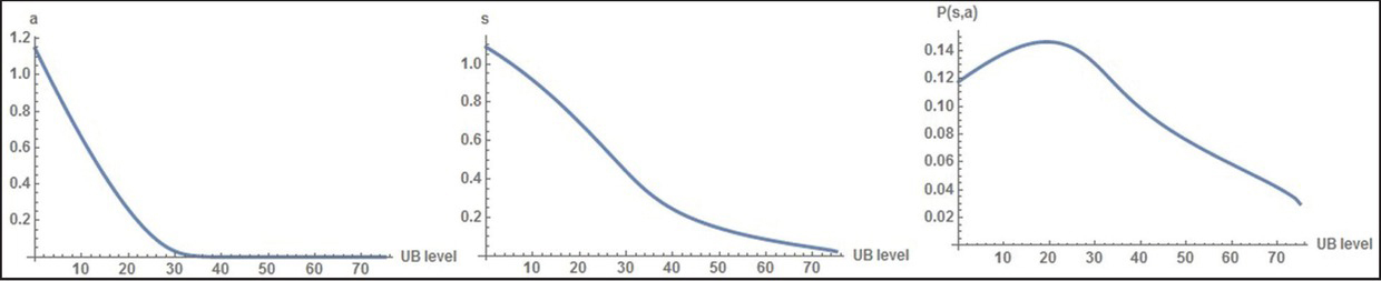
Figure 1
Baseline model [BM]. The three graphs show the level of a, s, and P(s, a), respectively, in the [BM] for different values of b. The functions and parameters are those of Table 1.
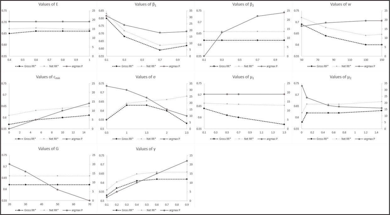
Figure 2
Sensitivity Analysis for the Baseline Model [BM]. These graphs report the results for 43 different specifications, all using the functions of Table 1. We take the parameterization of Table 1 and change one parameter at the time whose values are on the horizontal axis. “argmax P” is the level of b on the right vertical axis for which P(s, a) reaches the maximum.“Gross RR*” (respectively, “Net RR*”) gives the corresponding optimal gross (respectively, net) replacement rates on the left vertical axis: b/w (respectively, b/(w - 𝜏)).
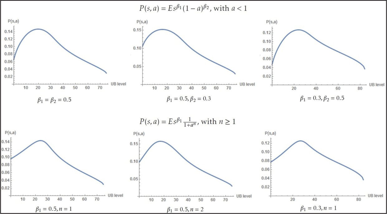
Figure 3
These graphs show the shape of the job-finding probability P(s, a) for different values of β1, β2 and β1, n, respectively. The other functions and parameters are those of Table 1.
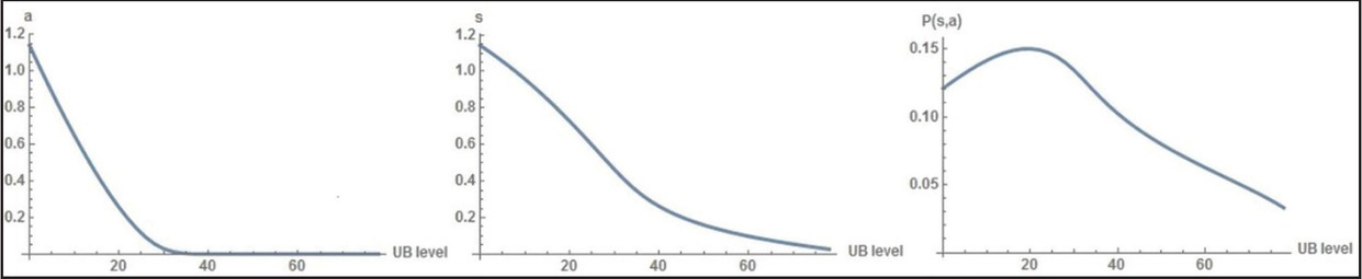
Figure 4
Finite Entitlement [FE]. The three graphs show the level of at, st and P(st, at), respectively, at the start of the unemployment spell, in the model [FE] for different values of b. The functions and parameters are those of Table 1, except for φ, which is now equal to zero. We set T = 200, the total quantity of time, and B = 100, the number of periods in which the agent is entitled to the flat benefit b.
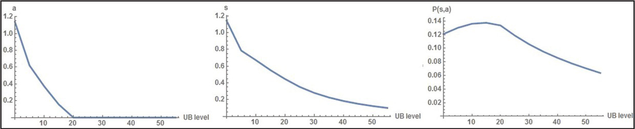
Figure 5
Incomplete Financial Markets [FM]. The three graphs show the level of at, st, and P(st, at), respectively, at the start of the unemployment spell in the model [FM] for different values of b. The functions and parameters are those of Table 1, except for φ, which is now equal to zero; moreover, we allow the agent to get indebted up to 200 (two times the wage) and we assume that the agent has to repay her debt at the end of the T = B = 200 periods.

Figure 6
Stochastic Wage Offers [SWO]. The three graphs show the level of at and st and the exit probability, respectively, at the start of the unemployment spell, in the model [SWO] for different values of b. The functions and parameters are those of Table 1, except for φ, which is now equal to zero, and σ = 2. We set T = B = 200, the total quantity of time. We assume that wages are Pareto distributed with parameters wmin = 66.66 and α = 3.
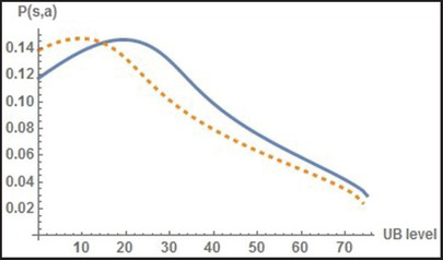
Figure 7
Cash Transfer Effect [BM]. This graph shows the job-finding probability P(s, a) for different values of b. The continuous line is generated with the functions and parameters of Table 1. The dashed line uses the same functions and parameters, the only difference being that the agent receives a transfer of 10 regardless of her employment status.
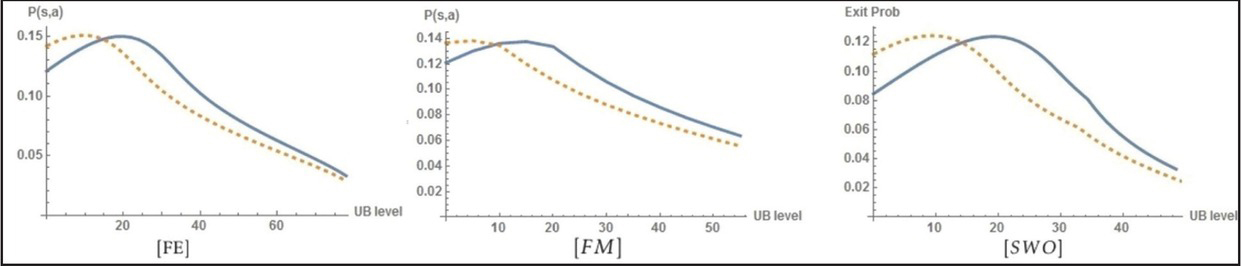
Figure 8
Cash Transfer Effect. These graphs show the job-finding probability P for different values of b, for the extensions: [FE], [FM], and [SWO]. The continuous line is generated with the functions and parameters discussed in the previous section for each model, and the dashed line is generated with the same parameters except for the fact that the agent receives a transfer of 10 regardless of her employment status.