
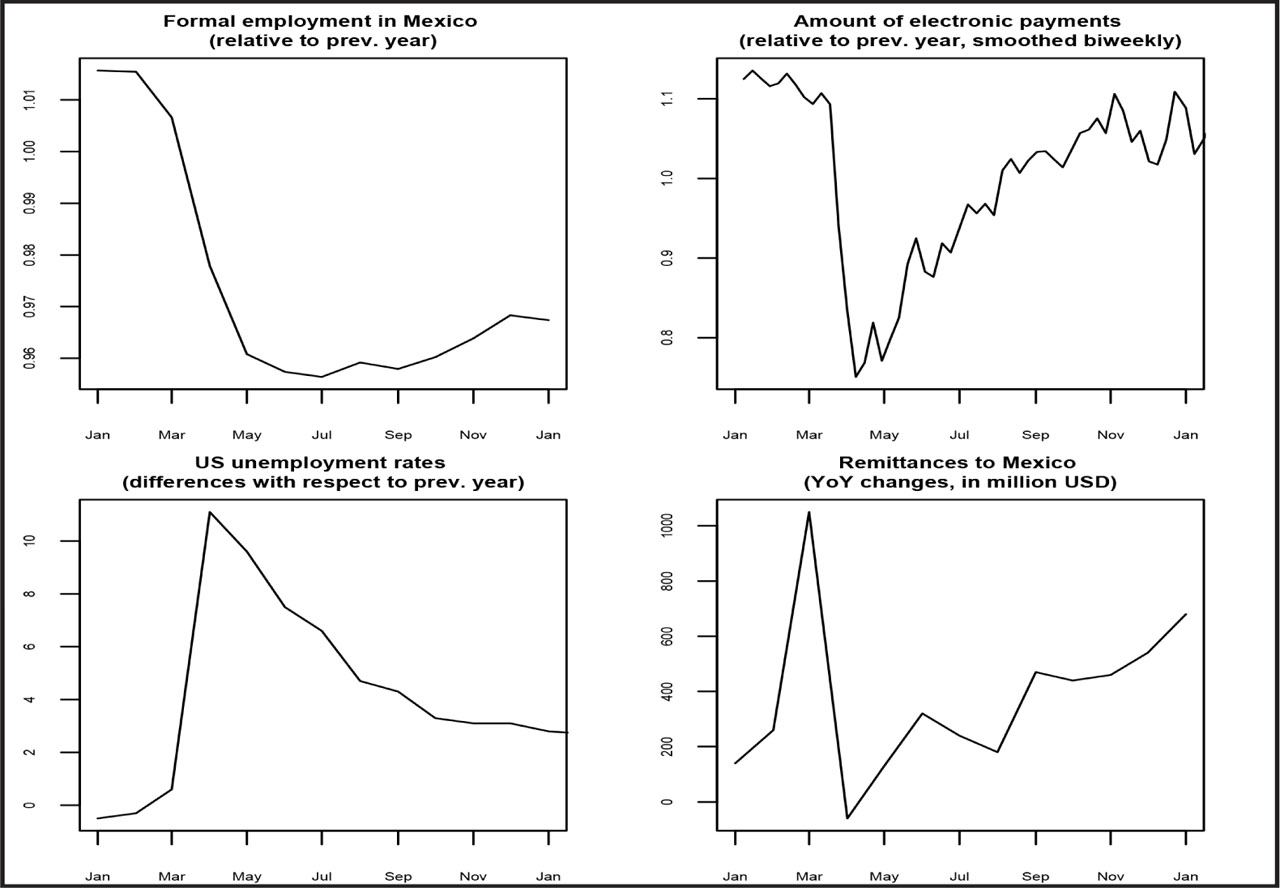
Figure 1
Trends in key variables during the pandemic year 2020.
Notes: Authors’ calculations. See Online Appendix 1 for a description of variables.
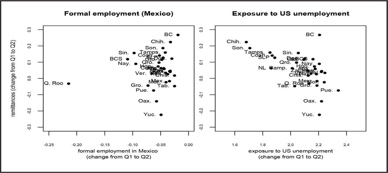
Figure 2
Remittances and employment situations in the US and Mexico (2020-Q2).
Notes: Authors’ calculations. Data on employment levels in Mexico (left) is based on data on formal employees from the Mexican Institute for Social Security (IMSS). Exposure to unemployment in the US is calculated from a weighted portfolio of migrants from each of the 31 Mexican states (not including Mexico City) across their destination in the US (right).
Table 1
Elasticity of remittances with respect to employment. State-level regressions
| Level of remittances (log) | ||||||
|---|---|---|---|---|---|---|
| I | II | III | IV | V | VI | |
| US unemployment exposure (log) | −1.02*** [0.20] | −1.00*** [0.21] | −0.50** [0.20] | −0.55*** [0.21] | −0.55*** [0.20] | −0.60* [0.32] |
| MX employment (log) | 0.19 [0.30] | −1.13*** [0.26] | −0.73 [0.60] | −0.56 [0.59] | ||
| Level of aggregation | state | state | state | state | state | state |
| Quarters covered | Q1, Q2 | Q1, Q2 | Q1, Q2, Q3, Q4 | Q1, Q2, Q3, Q4 | Q1, Q2, Q3, Q4 | Q1, Q2, Q3, Q4 |
| Interaction between weighted distance to diaspora and time | No | No | No | No | No | Yes |
| R2 | 0.43 | 0.44 | 0.51 | 0.55 | 0.56 | 0.58 |
| No. of observations | 62 | 62 | 124 | 124 | 120 | 120 |
[i] Notes: Authors’ calculations. Heteroscedasticity robust standard errors clustered at the state level in parenthesis. State−level regressions are run on 31 Mexican states (excluding Mexico City). Columns V and VI also exclude the state of Quintana Roo, a strong outlier in terms of employment and remittances. Stars denote significance at the 10% (*), 5% (**) and 1% (***) level. All results with municipality and quarter fixed effects.
Table 2
Elasticity of remittances with respect to employment. Municipal-level regressions
| Level of remittances (log) | ||||||
|---|---|---|---|---|---|---|
| I | II | III | IV | V | VI | |
| US unemployment exposure (log) | −0.98*** [0.17] | −0.98*** [0.17] | −0.58*** [0.14] | −0.58*** [0.14] | −0.58** [0.25] | −0.52** [0.17] |
| MX employment (log) | 0.08 [0.16] | −0.02 [0.12] | −0.02 [0.12] | −0.10 [0.99] | ||
| Level of aggregation | municipal | municipal | municipal | municipal | municipal | municipal |
| Quarters covered | Q1, Q2 | Q1, Q2 | Q1, Q2, Q3, Q4 | Q1, Q2, Q3, Q4 | Q1, Q2, Q3, Q4 | Q1, Q2, Q3, Q4 |
| Interaction between weighted distance to diaspora and time | No | No | No | No | Yes | No |
| Weighted by diaspora size | No | No | No | No | No | Yes |
| R2 | 0.21 | 0.22 | 0.24 | 0.24 | 0.27 | 0.22 |
| No. of observations | 770 | 770 | 1540 | 1540 | 1540 | 1540 |
[i] Notes: Authors’ calculations. Heteroscedasticity robust standard errors clustered at the municipal level in parenthesis. Municipal regressions are run on 385 municipalities with at least 50 thousand inhabitants. Stars denote significance at the 10% (*), 5% (**) and 1% (***) level. All results with municipality and quarter fixed effects.
Table 3
Effect of remittances on the amount of electronic payments. Two-stage least squares
| Amount of electronic payments (log) | ||||||
|---|---|---|---|---|---|---|
| I | II | III | IV | V | VI | |
| Amount of remittances (log) | 1.2*** [0.3] | 1.3*** [0.39] | 0.73*** [0.24] | 0.70*** [0.23] | 0.5** [0.2] | 0.55** [0.27] |
| Drop in workplace mobility (Google) | 0.0038 [0.0078] | |||||
| Drop in out-of-home events (GranData) | 0.40*** [0.12] | 0.32*** [0.067] | ||||
| Financial development | −0.017 [0.12] | 0.28 [0.42] | −0.29* [0.16] | |||
| Level of aggregation | state | state | municipal | municipal | municipal | municipal |
| Weighted by diaspora size | no | no | no | no | no | yes |
| Quarters covered | Q1, Q2 | Q1, Q2 | Q1, Q2 | Q1, Q2 | Q1, Q2, Q3, Q4 | Q1, Q2, Q3, Q4 |
| Weak instrument F-stat | 12 | 12 | 66 | 67 | 16 | 28 |
| # Observations | 62 | 62 | 772 | 772 | 1544 | 1544 |
[i] Second-step results instrumenting for remittances using migrants’ exposure to unemployment at the level of US states as an exogenous instrument. Heteroscedasticity robust standard errors clustered at the group level in parenthesis. Stars denote significance at the 10% (*), 5% (**) and 1% (***) level. All results with municipality (state) and year fixed effects. Limited information maximum likelihood estimates are provided in Online Appendix 6.
Online Appendix 1:
Data description
| Variable | Data Description | Level | Q1 | Q2 | Q3 | Q4 |
|---|---|---|---|---|---|---|
| Remittances | Inflow of total amount of remittances, in millions of USD.a) | state | 284.24 [248.65] | 298.88 [258.78] | 321.47 [258.48] | 320.73 [272.49] |
| municipal | 15.48 [19.09] | 16.26 [20.21] | 17.68 [22.38] | 17.49 [21.29] | ||
| MX employment levels | Number of formally employed persons registered with the Mexican Institute for Social Security IMSS, as a share of the adult population.b) c) | state | 0.23 [0.10] | 0.22 [0.10] | 0.22 [0.10] | 0.22 [0.10] |
| municipal | 0.18 [0.16] | 0.17 [0.15] | 0.17 [0.15] | 0.17 [0.15] | ||
| US unemployment exposure | Average exposure of migrants from each Mexican administrative entity i during quarter q using the weighting formula , where D denotes the share of diaspora from i in destination states k, and Unempl is the unemployment rate in destination state k. Data on migration corridors between Mexican municipalities of origin and US states of residence obtained from consular documents that register Mexican municipality of birth and US state of residence of all applicants.d) e) | state | 0.04 [0.00] | 0.13 [0.01] | 0.09 [0.01] | 0.07 [0.00] |
| municipal | 0.04 [0.00] | 0.13 [0.01] | 0.09 [0.01] | 0.07 [0.00] | ||
| Electronic payments | Total amount of electronic payments made via debit or credit card, geo-located at its point of sale. In millions of current Mexican Pesos.f) | state | 8845.12 [7268.58] | 6737.49 [5437.24] | 9170.64 [7452.55] | 9656.16 [7660.82] |
| municipal | 675.79 [1541.01] | 509.52 [1160.97] | 651.06 [1480.99] | 785.08 [1772.43] | ||
| Decrease in workplace mobility | Percentage drop in mobility between residence and workplace using location history from Google accounts on people's mobile devices, with respect to a median value for baseline days in the five-week period from January 3 to February 6, 2020.g) | state | −0.04 [0.02] | −0.36 [0.06] | −0.26 [0.04] | −0.20 [0.03] |
| Migrants’ exposure to decrease in workplace mobility | Average exposure of migrants from each Mexican administrative entity i to the drop in workplace mobility in their US states of residence k, using the same weighting formula as for exposure to unemployment.g) d) | state | −0.13 [0.00] | −0.36 [0.01] | −0.32 [0.00] | −0.27 [0.01] |
| municipal | −0.13 [0.00] | −0.36 [0.01] | −0.32 [0.01] | −0.27 [0.01] | ||
| Decrease in out-of-home events | Drop in the number of out-of-home events of cell-phone users, relative to the baseline data (March 2). The indicator first calculates the daily median for out-of-home events of all cell phone users, and then calculates the median over quarterly periods. Data before March 1 is set to zero and the fourth quarter ends on November 30.h) | municipal | 0.00 [0.00] | −0.21 [0.17] | −0.28 [0.15] | −0.32 [0.15] |
| Financial development | Number of bank accounts (sight deposits or “depósitos a la vista”) relative to the adult population.i) | state | 7.5 [10.6] | 6.9 [9.4] | 7.0 [9.5] | 7.1 [9.5] |
| municipal | 11.9 [21.2] | 10.7 [20.4] | 10.7 [20.1] | 10.6 [22.0] | ||
| Distance | Weighted average of direct distance in km from state capitals in Mexico to the state capital in the US state where migrants reside using the haversine formula. For exposure to unemployment, the average (weighted) distances between origin and destination is calculated depending on the distribution of migrants across the US.c) d) | state | 2016.13 [526.60] | |||
| municipal | 2183.45 [589.86] |
Sources:
Mean values and standard deviations in squared brackets for 31 states excluding the capital city of Mexico or 385 municipalities with a population of at least 50 thousand persons.
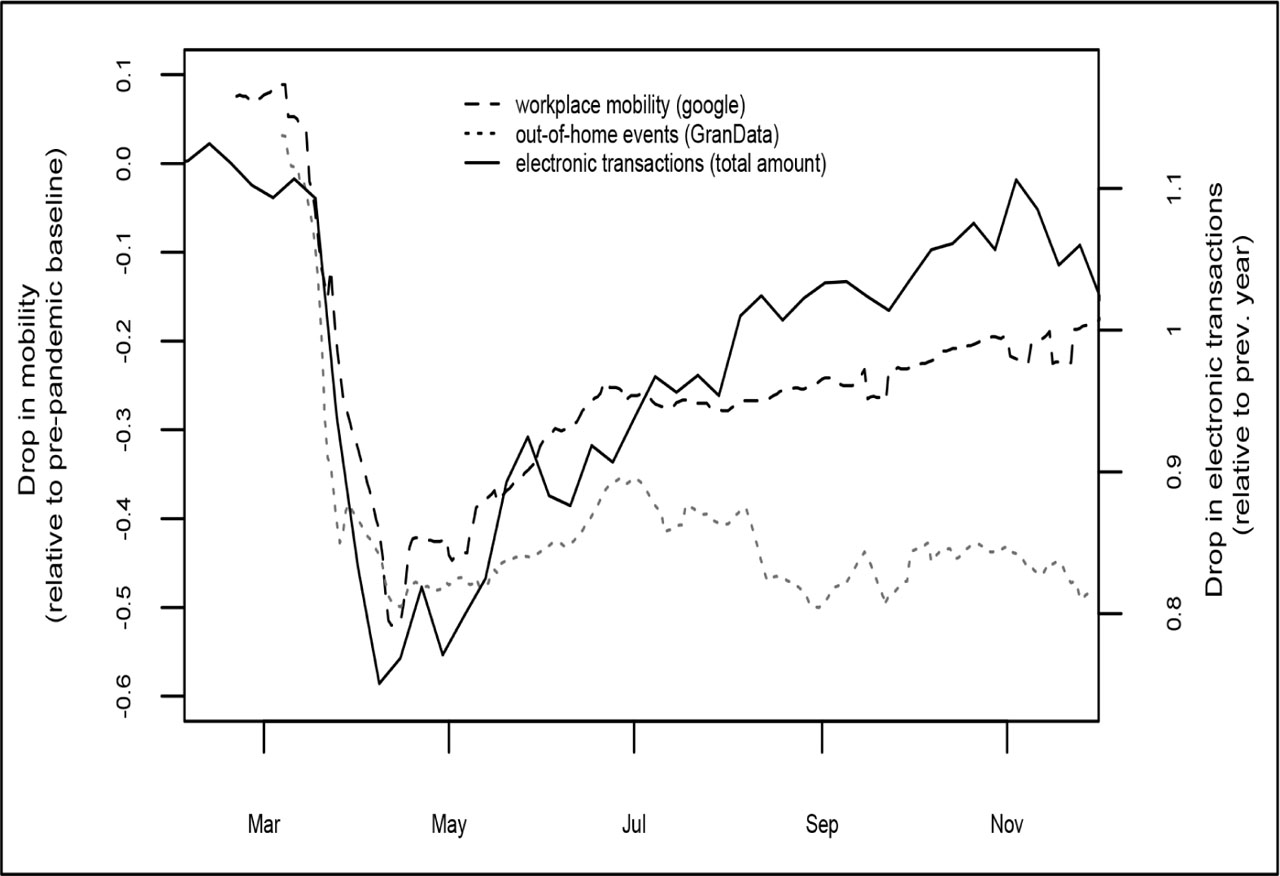
Online Appendix 2:
Decrease in mobility relative to baseline (left axis) and decrease in electronic transactions relative to previous year (right axis) during 2020 (daily values, smoothed)
See Online Appendix 1 for a description of variables.
Online Appendix 3:
Elasticity of remittances with respect to mobility drops. State-level regressions.
| Level of remittances (log) | |||||||
|---|---|---|---|---|---|---|---|
| I | II | III | IV | V | VI | VII | |
| Migrants exposure to decrease in workplace mobility | 8.33*** [2.19] | 8.11*** [2.10] | 3.30** [1.58] | 3.28* [1.63] | 3.24 [2.35] | ||
| Decrease in workplace mobility | 0.52* [026] | 0.48* [0.27] | 0.08 [0.24] | 0.05 [0.26] | 0.04 [0.28] | ||
| Level of aggregation | state | state | state | state | state | state | State |
| Quarters covered | Q1, Q2 | Q1, Q2 | Q1, Q2 | Q1, Q2, Q3, Q4 | Q1, Q2, Q3, Q4 | Q1, Q2, Q3, Q4 | Q1, Q2, Q3, Q4 |
| Interaction between weighted distance to diaspora and time | No | No | No | No | No | No | Yes |
| R2 | 0.35 | 0.26 | 0.40 | 0.50 | 0.49 | 0.50 | 0.52 |
| No. of observations | 62 | 62 | 62 | 124 | 124 | 124 | 124 |
Online Appendix 4:
Elasticity of remittances with respect to mobility drops. Municipality-level regressions.
| Level of remittances (log) | ||||||
|---|---|---|---|---|---|---|
| I | II | III | IV | V | VI | |
| Migrants exposure to decrease in workplace mobility | 7.93*** [1.16] | 8.24*** [1.16] | 2.76*** [0.87] | 2.76*** [0.87] | −0.47 [1.47] | |
| Decrease in out-of-home events | 0.09 [0.06] | 0.12* [0.06] | 0.20*** [0.07] | 0.19** [0.07] | ||
| Level of aggregation | municipal | municipal | municipal | municipal | municipal | municipal |
| Quarters covered | Q1, Q2 | Q1, Q2 | Q1, Q2 | Q1, Q2, Q3, Q4 | Q1, Q2, Q3, Q4 | Q1, Q2, Q3, Q4 |
| Interaction between weighted distance to diaspora and time | No | No | No | No | No | Yes |
| R2 | 0.18 | 0.09 | 0.20 | 0.23 | 0.24 | 0.27 |
| No. of observations | 772 | 772 | 772 | 1544 | 1544 | 1544 |
Online Appendix 5:
Remittances and electronic payments. Non-instrumented OLS
| Amount of electronic payments (log) | ||||||
|---|---|---|---|---|---|---|
| Level of remittances (log) | 0.80*** [0.17] | 0.69*** [0.14] | 0.34*** [0.06] | 0.28*** [0.06] | 0.03** [0.01] | 0.01 [0.02] |
| Decrease in workplace mobility | 0.72 [0.55] | |||||
| Decrease in out-of-home events | 0.44*** [0.07] | 0.29*** [0.04] | ||||
| Level of aggregation | state | state | municipal | municipal | municipal | municipal |
| Quarters covered | Q1, Q2 | Q1, Q2 | Q1, Q2 | Q1, Q2 | Q1, Q2, Q3, Q4 | Q1, Q2, Q3, Q4 |
| R2 | 0.89 | 0.91 | 0.47 | 0.57 | 0.66 | 0.70 |
| F-stat | 116 | 106 | 167 | 144 | 562 | 299 |
| No. of observations | 62 | 62 | 772 | 772 | 1544 | 1544 |
Online Appendix 6:
Effect of remittances on the amount of electronic payments. LIML estimation
| Amount of electronic payments (log) | ||||||
|---|---|---|---|---|---|---|
| Amount of remittances (log) | 1.16*** [0.21] | 1.17*** [0.21] | 0.73*** [0.17] | 0.72*** [0.16] | 0.50*** [0.17] | 0.50*** [0.167] |
| Decrease in workplace mobility | 0.48 [0.51] | |||||
| Decrease in out-of-home events | 0.40*** [0.08] | 0.16** [0.06] | ||||
| Level of aggregation | state | state | municipal | municipal | municipal | municipal |
| Quarters covered | Q1, Q2 | Q1, Q2 | Q1, Q2 | Q1, Q2 | Q1, Q2, Q3, Q4 | Q1, Q2, Q3, Q4 |
| Weak instrument F-stat LIML CI | 12 [0.75, 1.56] | 14 [0.76, 1.58] | 66 [0.39, 1.06] | 67 [0.41, 1.04] | 16 [0.17, 0.83] | 16 [0.18, 0.83] |
| No. of observations | 62 | 62 | 772 | 772 | 1544 | 1544 |
[i] Second-step results instrumenting for remittances using migrants exposure to unemployment at the level of US states as an exogenous instrument. Heteroscedasticity robust standard errors clustered at the group level in parenthesis. Stars denote significance at the 10% (*), 5% (**) and 1% (***) level. All results with municipality (state) and year fixed effects. Weak instruments confidence intervals clustered at the group level in brackets estimated as in Mikusheva and Poi (2006).