
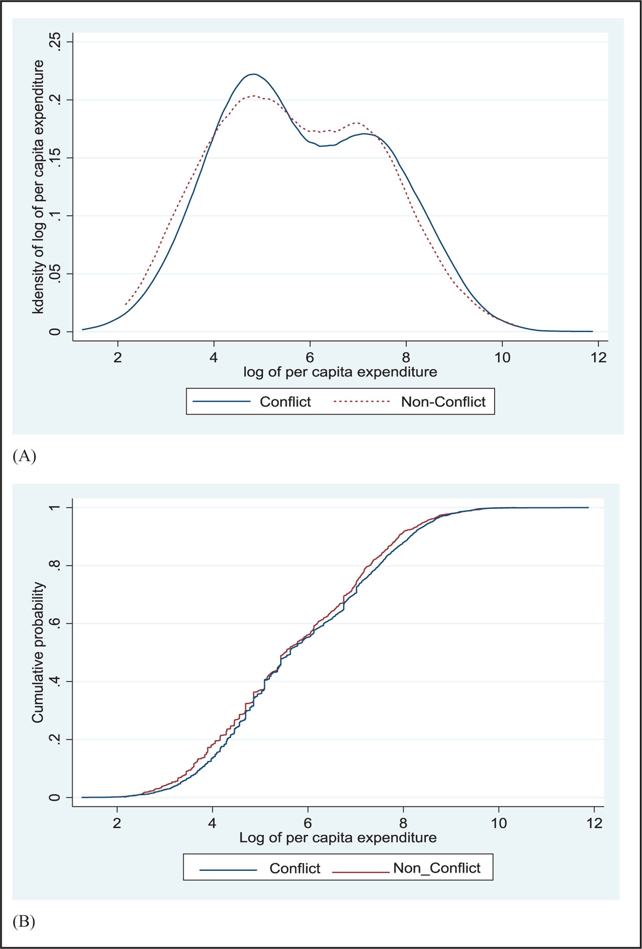
Figure 1
(A) The Density Functions of Household Expenditure by Conflict Exposure (1989). (B) The Distribution Functions of Household Expenditure by Conflict Exposure (1989).
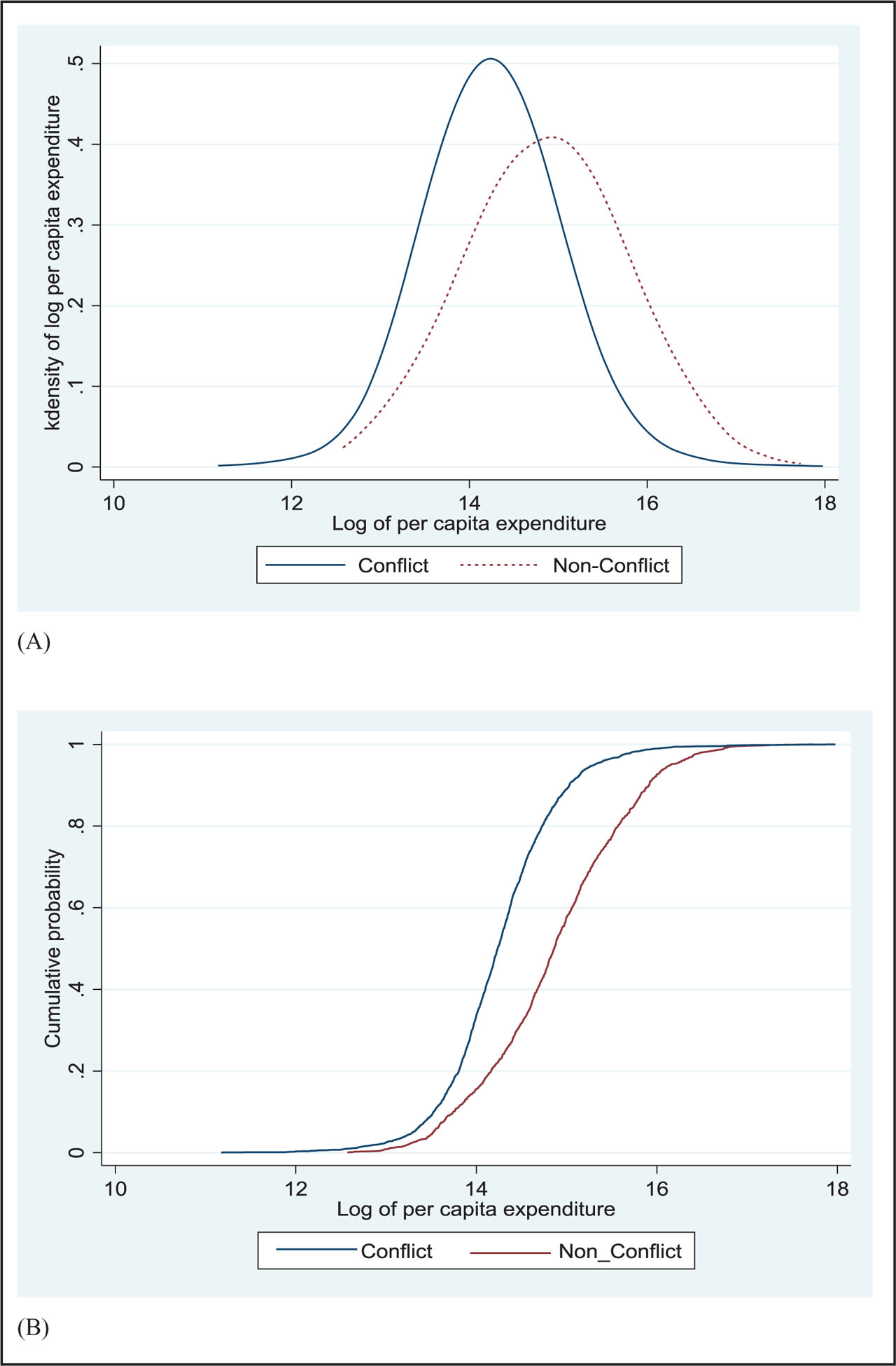
Figure 2
(A) The Density Functions of Household Expenditure by Conflict Exposure (2003). (B) The Distribution Functions of Household Expenditure by Conflict Exposure (2003).
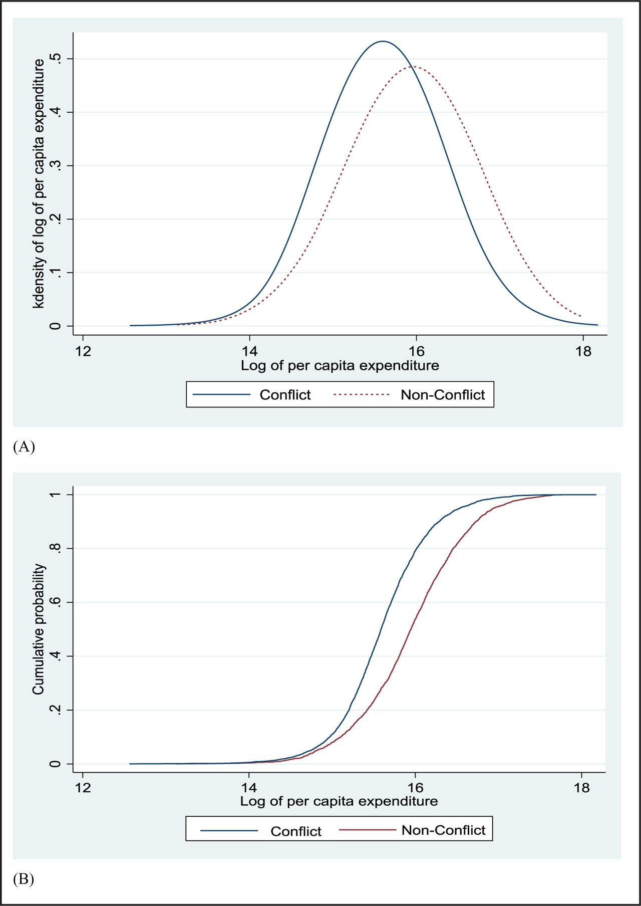
Figure 3
(A) The Density Functions of Household Expenditure by Conflict Exposure (2011). (B) The Distribution Functions of Household Expenditure by Conflict Exposure (2011).
Table 1
Sierra Leone Household Expenditure Percentile Ratios by Conflict Exposure
| 90th–10th | 90th–50th | 50th–10th | |
|---|---|---|---|
| 50th | 50th | 50th | |
| 1989: | |||
| Overall | 10.1315 | 9.3909 | 0.7406 |
| Conflict | 8.1130 | 7.2757 | 0.8373 |
| Non-conflict | 9.3891 | 8.6631 | 0.7260 |
| Change | −1.2761 | −1.3874 | 0.1113 |
| 2003: | |||
| Overall | 2.5614 | 2.0107 | 0.5507 |
| Conflict | 1.6637 | 1.1458 | 0.5178 |
| Non-conflict | 3.2174 | 2.6255 | 0.5919 |
| Change | −1.5537 | −1.4797 | −0.0741 |
| 2011: | |||
| Overall | 1.7592 | 1.2537 | 0.5055 |
| Conflict | 1.4517 | 0.9520 | 0.4994 |
| Non-conflict | 1.8487 | 1.3408 | 0.5078 |
| Change | −0.3970 | −0.3888 | −0.0084 |
| Raw difference-in-difference | |||
| D-i-D1 (2003–1989) | −0.2776 | −0.0923 | −0.1854 |
| D-i-D2 (2011–1989) | 0.8791 | 0.9986 | −0.1197 |
[i] Notes: “Change” denotes the difference in outcomes between the conflict and non-conflict affected zones; see Table 2 for the relevant sample sizes used to compute the relevant summary statistics. D-i-D1 and D-i-D2 are the raw difference-in-differences between 2003/1989 and 2011/1989; the 2003 and 2011 expenditure values were based on a new currency code introduced in Sierra Leone, which replaced the previous denomination in cents to Leones (Le). The ISO 4217 code introduced the currency change from 100 cents to 1 Le. This accounts for the change in absolute magnitudes reported in 2003 and 2011 compared to 1989.
Table 2
Standard Deviation of Log of Household Expenditure by Conflict Exposure
| 1989 | 2003 | 2011 | |
|---|---|---|---|
| Standard deviation: | |||
| Overall | 1.4596 | 0.7627 | 0.6121 |
| Conflict | 1.5661 | 0.6013 | 0.5602 |
| Non-conflict | 1.3997 | 0.8608 | 0.6230 |
| Change | 0.1664 | −0.2595 | −0.0628 |
| Raw difference-in-difference | |||
| D-i-D1 (2003–1989) | n/a | −0.4259 | n/a |
| D-i-D2 (2011–1989) | n/a | n/a | −0.2292 |
| Observations: | 3439 | 3702 | 6763 |
| Treatment | 1167 | 1666 | 4041 |
| Control | 2272 | 2036 | 2722 |
[i] Notes: “Change” denotes the difference in standard deviations between the conflict and non-conflict affected zones;
[ii] D-i-D1 and D-i-D2 are the raw differences-in-difference between 2003/1989 and 2011/1989 respectively; n/a denotes not applicable.
Table 3
Gini Coefficient for Household Expenditure by Conflict Exposure
| 1989 | 2003 | 2011 | |
|---|---|---|---|
| Gini Coefficient: | |||
| Overall | 0.672*** (0.008) | 0.442*** (0.008) | 0.3380*** (0.003) |
| Conflict | 0.659*** (0.009) | 0.377*** (0.012) | 0.302*** (0.005) |
| Non-conflict | 0.677*** (0.011) | 0.434*** (0.010) | 0.344*** (0.004) |
| Change | −0.017 (0.014) | −0.057*** (0.016) | −0.042*** (0.006) |
| Difference-in-difference | |||
| D-i-D1 (2003–1989) | n/a | −0.040** (0.021) | n/a |
| D-i-D2 (2011–1989) | n/a | n/a | −0.025 (0.015) |
| Observations: | 3439 | 3702 | 6763 |
| Treatment | 1167 | 1666 | 4041 |
| Control | 2272 | 2036 | 2722 |
Notes:
“Change” denotes the difference between conflict and non-conflict zones; bootstrapped standard errors with 250 replications are reported in parenthesis; D-i-D1 and D-i-D2 are the raw differences-in-difference between 2003/1989 and 2011/1989, respectively; n/a denotes not applicable; the significance levels are denoted as
Table 4
Log Household Expenditure Differentials between Conflict and Non-conflict Zones at the Mean and Selected Quantiles
| Mean and selected percentiles | 1989 | 2003 | 2011 |
|---|---|---|---|
| Mean | 0.0526 (0.0621) | −0.5447*** (0.0502) | −0.3318*** (0.0403) |
| 10th | −0.2506*** (0.0611) | −0.1923*** (0.0552) | −0.0037 (0.0026) |
| 25th | −0.1037*** (0.0649) | −0.3762*** (0.0413) | −0.1453*** (0.1806 |
| 50th | −0.0000 (0.1028) | −0.4798*** (0.0354) | −0.3444*** (0.0193) |
| 75th | 0.3696*** (0.0777) | −0.6325*** (0.0375) | −0.4967*** (0.0217) |
| 90th | 0.1589** (0.0813) | −0.7974*** (0.0528) | −0.5485*** (0.0317) |
| Observations: | 3439 | 3702 | 6763 |
| Treatment | 1167 | 1666 | 4041 |
| Control | 2272 | 2036 | 2722 |
Table 5
Summary Statistics of Household Characteristics by Conflict Exposure
| 1989 | 2003 | 2011 | ||||
|---|---|---|---|---|---|---|
| Conflict | Non-conflict | Conflict | Non-conflict | Conflict | Non-conflict | |
| Head's characteristics: | ||||||
| Age | 44.43 (11.44) | 43.75 (11.91) | 46.80 13.99 | 46.19 14.29 | 45.70 14.68 | 45.49 13.83 |
| Age squared | 2104.39 (1119.90) | 2056.01 (1193.83) | 2386.05 1461.48 | 2337.35 1483.03 | 2304.35 1515.08 | 2259.99 1409.94 |
| Gender: | ||||||
| Male | 0.87 | 0.85 | 0.82 | 0.80 | 0.72 | 0.74 |
| Female | 0.13 | 0.15 | 0.18 | 0.20 | 0.26 | 0.24 |
| Education: | ||||||
| Primary | 0.68 | 0.56 | 0.09 | 0.08 | 0.08 | 0.09 |
| High | 0.32 | 0.44 | 0.02 | 0.04 | 0.12 | 0.11 |
| Secondary | - | - | 0.12 | 0.20 | 0.05 | 0.21 |
| No education | - | - | 0.75 | 0.64 | 0.76 | 0.59 |
| Marital Status: | ||||||
| Married | 0.92 | 0.92 | 0.84 | 0.79 | 0.81 | 0.77 |
| Cohabit | 0.04 | 0.06 | 0.01 | 0.01 | 0.01 | 0.01 |
| Other status | 0.05 | 0.09 | 0.15 | 0.16 | 0.15 | 0.15 |
| Single | 0.02 | 0.02 | 0.01 | 0.03 | 0.03 | 0.06 |
| Tribes: | ||||||
| Mende | - | - | 0.38 | 0.37 | - | - |
| Temne | - | - | 0.24 | 0.23 | - | - |
| Other tribes | - | - | 0.38 | 0.40 | - | - |
| Religion: | ||||||
| Muslim | - | - | - | - | 0.78 | 0.74 |
| Christian | - | - | - | - | 0.21 | 0.25 |
| Other religions | - | - | - | - | 0.01 | 0.01 |
| Other Characteristics: | ||||||
| Urban | 0.33 | 0.35 | 0.30 | 0.40 | 0.17 | 0.48 |
| Dependency ratio | 0.99 | 0.91 | 0.95 | 0.94 | 1.08 | 1.15 |
| 0.91 | 0.93 | 0.90 | 0.87 | 1.03 | 1.16 | |
| Household size | 6.16 | 5.29 | 6.28 | 6.11 | 5.64 | 5.61 |
| 4.05 | 3.34 | 2.61 | 2.85 | 2.47 | 2.67 | |
| Household size squared | 54.37 | 39.14 | 46.28 | 45.43 | 37.98 | 38.76 |
| 69.71 | 50.22 | 40.48 | 45.55 | 35.66 | 42.79 | |
| Sample size | 1167 | 2272 | 1666 | 2036 | 2722 | 4041 |
[i] Notes: Standard deviations for continuous variables reported in parenthesis; conflict exposure refers to whether a household is located within the conflict-affected chiefdoms, defined as being subject to >8 years of rebel occupation.
Table 6
The Impact of Conflict on the Distribution of Expenditure using the Gini Coefficient
| Estimation Methods | Conflict Exposure | ||
|---|---|---|---|
| 1989 | 2003 | 2011 | |
| (1) Unweighted | 0.0039 (0.0156) | −0.0908*** (0.0126) | −0.0051 (0.0050) |
| (2) Weighted | 0.0025 (0.0140) | −0.0804*** (0.0125) | 0.0037 (0.0048) |
| (3) PS regressor | 0.0039 (0.0197) | −0.0912*** (0.0152) | −0.0030 (0.0050) |
| (4) Matching (ATT) | 0.0108 (0.0184) | −0.0552*** (0.0183) | 0.0048 (0.0081) |
| (5) IPW (ATT) | 0.0031 (0.0147) | −0.0834*** (0.0125) | −0.0001 (0.0048) |
| Observations: | 3439 | 3702 | 6763 |
| Treatment | 1167 | 1666 | 4041 |
| Control | 2272 | 2036 | 2722 |
Notes:
The estimates reported for (1) to (3) relate to the regression estimate from Eq. (2). Specifically, the different regression results are based on the following: (1) OLS without regression weights; (2) OLS with the propensity score as regression weights; (3) the propensity score is included as an additional covariate in the regression; (4) uses the propensity score matching technique with the RIF-based Gini; (5) uses the inverse probability weighting technique with the RIF-based Gini. Standard errors are reported in parentheses; the significance levels are defined as:
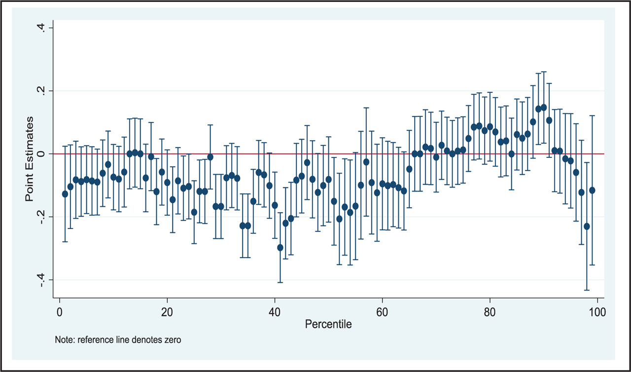
Figure 4
Point Estimates and 95% Confidence Intervals for Quantile Conflict Treatment Effects (1989).
Notes: The QTT point estimates are derived using expression Eq. (4) in the text with the variables included in the local logistic treatment assignment equation described in the notes to Table 7. The 95% confidence intervals are based on bootstrapping with 250 replications. The mean estimate is obtained using a regression model containing the same set of covariates.
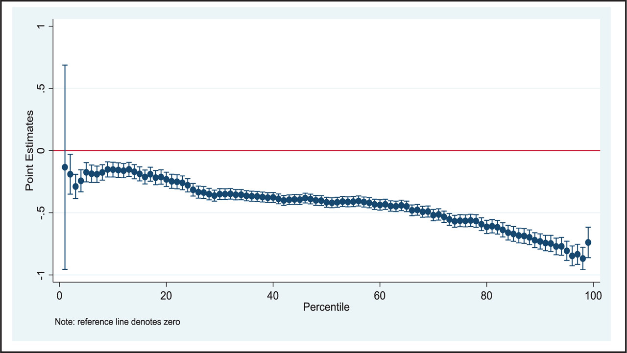
Figure 5
Point Estimates and 95% Confidence Intervals for Quantile Conflict Treatment Effects (2003).
Notes: The QTT point estimates are derived using the expression in Eq. (4) in the text with the variables included in the local logistic treatment assignment equation described in the notes to Table 7. The 95% confidence intervals are based on bootstrapping with 250 replications. The mean estimate is obtained using a regression model containing the same set of covariates.
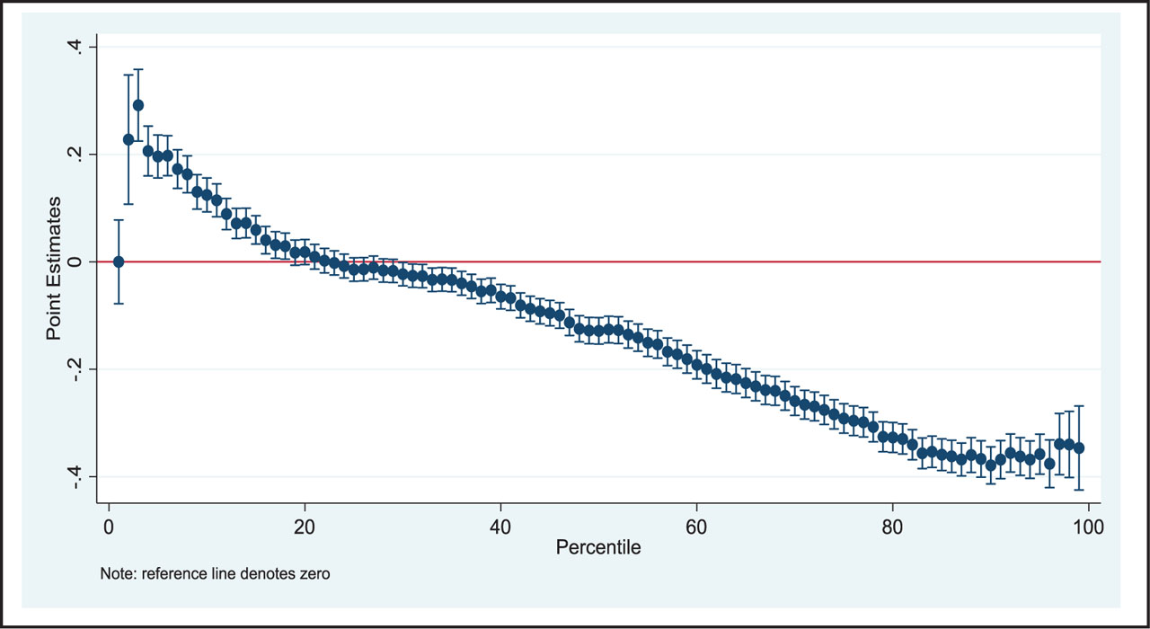
Figure 6
Point Estimates and 95% Confidence Intervals for Quantile Conflict Treatment Effects (2011).
Notes: The QTT point estimates are derived using the expression in Eq. (4) in the text with the variables included in the local logistic treatment assignment equation described in the notes to Table 7. The 95% confidence intervals are based on bootstrapping with 250 replications. The mean estimate is obtained using a regression model containing the same set of covariates.
Table 7
Mean and Quantile Treatment Effects using the Log of Household Expenditure
| Mean | 10th | 25th | 50th | 75th | 90th | |
|---|---|---|---|---|---|---|
| 1989: | ||||||
| Conflict exposure | −0.0831 (0.0588) | −0.0560 (0.0825) | −0.1853*** (0.0769) | −0.0813 (0.1476) | −0.0115 (0.0876) | 0.1183 (0.1213) |
| Observations | 3,439 | 3,422 | 3422 | 3422 | 3422 | 3422 |
| 2003: | ||||||
| Conflict exposure | −0.4437*** (0.0531) | −0.1624*** (0.0547) | −0.3065*** (0.0635) | −0.3974*** (0.0392) | −0.5515*** (0.0336) | −0.6821*** (0.0579) |
| Observations | 3702 | 3702 | 3702 | 3702 | 3702 | 3702 |
| 2011: | ||||||
| Conflict exposure | −0.2601*** (0.0498) | 0.0786** (0.0332) | −0.0390** (0.0189) | −0.1401*** (0.0161) | −0.2726*** (0.0269) | −0.3013*** (0.0388) |
| Observations | 6763 | 6763 | 6763 | 6763 | 6763 | 6763 |
Notes:
Seventeen observations were trimmed from the QTT analysis for 1989 with propensity scores below 0.0001 and none from the two subsequent years. The treatment assignment equation contains the following controls: head of household age and its quadratic, head of household gender, head of household education and marital status, household size and it quadratic; household dependency ratio; the household's settlement type; and a selection of interaction variables (see Table A2.7 in Appendix II). Bootstrapped standard errors are reported in parentheses with 250 replications; the significance levels are denoted by
Table 8
The Impact of Conflict on the Gini Coefficient using Alternative Conflict Measures
| Estimation Methods | Exposure (7 years cut-off) | Exposure (above median dummy) | ||||
|---|---|---|---|---|---|---|
| 1989 | 2003 | 2011 | 1989 | 2003 | 2011 | |
| (1) Unweighted | 0.0040 (0.0157) | −0.0912*** (0.0128) | −0.0055 (0.0052) | 0.0257 (0.0185) | −0.0952*** (0.0141) | −0.0147** (0.0051) |
| (2) Weighted | 0.0030 (0.0141) | −0.0805*** (0.0131) | 0.0037 (0.0038) | 0.0263 (0.0214) | −0.0811*** (0.0138) | −0.0074 (0.0046) |
| (3) PS regressor | 0.0041 (0.0198) | −0.0924*** (0.0157) | −0.0035 (0.0052) | 0.0254 (0.0189) | −0.0954*** (0.0152) | −0.0139* (0.0050) |
| (4) Matching (ATT) | 0.0109 (0.0188) | −0.0563*** (0.0189) | 0.0051 (0.0084) | 0.0365 (0.0194) | −0.0768*** (0.0238) | −0.0758 (0.0571) |
| (5) IPW (ATT) | 0.0031 (0.0145) | −0.0845*** (0.0132) | −0.0001 (0.0056) | 0.0253 (0.0174) | −0.0827*** (0.0138) | −0.0168** (0.0053) |
| Observations: | 3439 | 3702 | 6763 | 3439 | 3702 | 6763 |
| Treatment | 1167 | 1666 | 4041 | 1954 | 1965 | 4041 |
| Control | 2272 | 2036 | 2722 | 1485 | 1737 | 2722 |
Note:
The conflict exposure measure is based on either an occupation of ≥7 years or whether or not the deaths per chiefdom were above the national median; the different regression results are based on the following: (1) OLS without regression weights; (2) OLS with the propensity scores as regression weights; (3) the propensity score is included as an additional covariate in the regression model; (4) uses the propensity score matching technique; (5) uses the inverse probability weighting technique. Robust standard errors are reported in parentheses; the significance levels are denoted by
Table 9
OLS and Quantile Treatment Effects using Log Household Expenditure – Conflict Exposure (using ≥7 years of rebel occupation as the cut-off)
| Mean | 10th | 25th | 50th | 75th | 90th | |
|---|---|---|---|---|---|---|
| 1989: | ||||||
| Conflict exposure | −0.0841 (0.0598) | −0.0520 (0.0885) | −0.1803*** (0.0716) | −0.0822 (0.1480) | −0.0120 (0.0854) | 0.1180 (0.1214) |
| Observations | 3439 | 3439 | 3439 | 3439 | 3439 | 3439 |
| 2003: | ||||||
| Conflict exposure | −0.1468*** (0.0485) | −0.0149 (0.0500) | −0.0542 (0.0358) | −0.0928*** (0.0318) | −0.2208*** (0.0384) | −0.4167*** (0.0512) |
| Observations | 3702 | 3702 | 3702 | 3702 | 3702 | 370 |
| 2011: | ||||||
| Conflict exposure | −0.1607*** (0.0377) | −0.0974** (0.0264) | −0.0934*** (0.0265) | −0.1065*** (0.0217) | −0.1563*** (0.0285) | −0.2119*** (0.0456) |
| Observations | 6763 | 6763 | 6763 | 6763 | 6763 | 6763 |
Notes:
The treatment assignment equation contains the following controls: head of household age and its quadratic, head of household gender, head of household education and marital status, household size and it quadratic; household dependency ratio; the household's settlement type; and a selection of interaction variables. Bootstrapped standard errors are reported in parentheses with 250 replications; the significance levels are denoted by
Table 10
OLS and Quantile Treatment Effects using Log Household Expenditure – Conflict Exposure using Conflict Deaths per Chiefdom Above the Median
| Mean | 10th | 25th | 50th | 75th | 90th | |
|---|---|---|---|---|---|---|
| 1989: | ||||||
| Conflict exposure | 0.1043 (0.0411) | −0.0505 (0.0692) | 0.0661 (0.0776) | 0.2283 (0.1421) | 0.4849*** (0.0649) | 0.2627*** (0.0763) |
| Observations | 3439 | 3439 | 3439 | 3439 | 3439 | 3439 |
| 2003: | ||||||
| Conflict exposure | −0.1468*** (0.0485) | −0.0255 (0.0481) | −0.0761 (0.0379) | −0.1594*** (0.0309) | −0.3416*** (0.0451) | −0.5074*** (0.0517) |
| Observations | 3702 | 3702 | 3702 | 3702 | 3702 | 3702 |
| 2011: | ||||||
| Conflict exposure | −0.1607*** (0.0377) | −0.0974** (0.0264) | −0.0934*** (0.0265) | −0.1065*** (0.0217) | −0.1563*** (0.0285) | −0.2119*** (0.0456) |
| Observations | 6763 | 6763 | 6763 | 6763 | 6763 | 6763 |
Notes:
The treatment assignment equation contains the following controls: head of household age and its quadratic, head of household gender, head of household education and marital status, household size and it quadratic; household dependency ratio; the household's settlement type; and a selection of interaction variables. Bootstrapped standard errors are reported in parentheses with 250 replications; the significance levels are denoted by
Table 11
The Impact of Conflict on the Gini Coefficient using Self-reported Conflict Events
| Conflict Events | |
|---|---|
| Estimation Methods | 2003 |
| (1) Unweighted | −0.0802*** (0.0183) |
| (2) Weighted | −0.0751*** (0.0214) |
| (3) PS regressor | −0.0800*** (0.0169) |
| (4) Matching (ATT) | −0.0691*** (0.0265) |
| (5) IPW (ATT) | −0.0736*** (0.0395) |
| Observations: | 3696 |
| Treatment | 1319 |
| Control | 2377 |
Note:
The conflict measure is self-reported (see text). The estimates reported for (1) to (3) relate to the regression estimate ^ from Eq. (2). Specifically, the different regression results are based on the following: (1) OLS without regression weights; (2) OLS with the propensity score as regression weights; (3) the propensity score is used as an additional covariate in the regression model; (4) uses the propensity score matching technique; (5) uses the inverse probability weighting technique. Standard errors in parentheses; the significance levels are denoted by
Table 12
OLS and Quantile Treatment Effects of Conflict on Log Household Expenditure using Self-reported Conflict Events
| OLS | 10th | 25th | 50th | 75th | 90th | |
|---|---|---|---|---|---|---|
| 2003: | ||||||
| Conflict events | −0.446*** (0.0460) | −0.1796*** (0.0561) | −0.2906*** (0.0582) | −0.3885*** (0.0375) | −0.5469*** (0.0381) | −0.6834*** (0.0576) |
| Observations | 3696 | 3696 | 3696 | 3696 | 3696 | 3696 |
Notes:
The conflict measure is self-reported (see text). The treatment assignment equation contains the following controls: head of household age and its quadratic, head of household gender, head of household education and marital status, household size and it quadratic; household dependency ratio; the household's settlement type; and a selection of interaction variables. Bootstrapped standard errors are reported in parentheses with 250 replications; the significance levels are denoted by
Table A1
Chiefdom Allocation to “Treatment” and “Control” Group
| Years in Survey | Chiefdoms in Treatment Group | Chiefdoms in Control Group |
|---|---|---|
| 1989, 2003, and 2011 | Eastern Regions: Biriwa Bombali Shebro Bum Dama Fiama Jawie Mandu Lower Bambara Nimikoro Njaluahun Nongowa Simbaru Small Bo Tankoro Northern Region Gbanti-Kamaranka Gbendembu Ndowahun Gbinleh Dixing Southern Region: Jong Kaiyamba Panga Kabone Valunia Bumpeh Fakunya Northern Region: Koya Magbema Makari Gbanti Malal Mambolo Masungbala Sanda Loko Sella Limba | Eastern Region: Malegohun Gbense Gorama Kono Northern Region: Paki Masabong Samu Dembelia Sinkunia Follosaba Dembelia Sulima Wara Wara Yagala Kaffu Bullom Lokomasama Maforki Marampa Gbonkolenken Kholifa Mabang Kunike Barina Southern Region: Bagbo Baoma Jaiama Bongor Kakua Komboya Tikonko Imperi Kpanga Kemo Bumpeh Upper Banta Barri Western Area Mountain York Rural Waterloo Central 1 Central 2 East 1 East 2 East 3 West 1 West 2 West 3 |
| 2003 and 2011 only | Eastern Regions: Kissi Kama Luawa Penguia Yawei Gorama Mende Langrama Gbane Kamara Lei Nimiyama Sandor Northern Region: Safroko Limba Sanda Tendaren Tambakka Tonko Limba Mongo Neya Sengbe Bureh Kasseh Buya Romende Dibia Sanda Magbolontor Southern Region: Jong Nongoba Bullom Kamajei Kongbora Makpele Pejeh Soro Gbema | Eastern Regions: Kissi Tongi Kpeje Bongre Kpeje West Dodo Gaura Kandu Lekpeama Nomo Tunkia Wandor Mafindor Soa Malema Nomo Niawa Northern Region: Libeisaygahun Magbaimba Ndorhahun Kasunko Nieni Wara Wara Bafodia Masimera Kafe Simira Kalansogoia Tane Paki Masonbong Braiama Diang Southern region: Bumpe Ngawo Niawa Lenga Bendu Cha Sogbini Bagruwa Kagboro Kowa Lower Banta Timdale Gallinas Peri Mano Sakrim Yakemo Kpukumu Krim Badjia Bagbo Wunde Kwamebi Krim- Beduma Sittia- Yonni Yawbeko- Talia Dasse Kori Ribbi Kpaka Sowa |
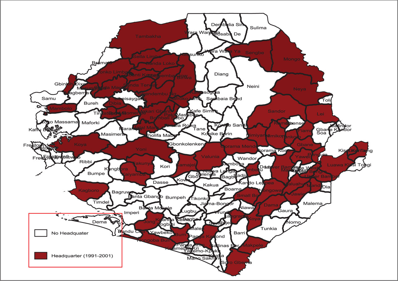
Figure A1
Conflict Exposure by Rebel Occupation based on the Presence of Rebel Headquarters by Chiefdom.
Table A2.1
Kolmogorov–Smirnov Tests for Equality of Distributions by Conflict Exposure
| Years | Distance | Exact Prob-value |
|---|---|---|
| 1989 | 0.0492 | 0.121 |
| 2003 | 0.2689 | 0.000 |
| 2011 | 0.2515 | 0.000 |
[i] Notes: The null hypothesis is that the empirical distribution functions across treatment (conflict) and control (non-conflict) groups are equal. The “Distance” is the maximum vertical distance between the CDFs for the two groups and the prob-value is used to determine whether the distance is statistically significant.
Table A2.2
Logistic Treatment Assignment Model for Conflict Exposure and Conflict Events
| 1989 | 2003 | 2011 | ||
|---|---|---|---|---|
| Conflict Exposure | Conflict Exposure | Conflict Events | Conflict Exposure | |
| Age of head | 0.00789 (0.0199) | 0.0183 (0.0138) | 0.0275* (0.0159) | −0.0364*** (0.0104) |
| Age of head square | −0.000157 (0.000200) | −0.000162 (0.000131) | −0.000195 (0.000151) | 0.000330*** (0.00010) |
| Head being male | 0.206 (0.126) | −0.192 (0.154) | 0.620*** (0.185) | −0.0641 (0.0826) |
| Head married | −0.0147 (0.163) | −0.164 (0.166) | −0.568*** (0.208) | −0.0602 (0.0991) |
| Dependency ratio | 0.0241 (0.0554) | 0.0530 (0.0499) | −0.0995* (0.0589) | −0.0231 (0.0308) |
| Urban | −0.118 (0.149) | −0.978*** (0.246) | −1.082*** (0.284) | −2.127*** (0.201) |
| Head with prim educ | 0.535*** (0.0804) | −0.0175 (0.160) | 0.882*** (0.224) | −0.228* (0.125) |
| Head with higher educ | - | −0.469** (0.206) | −0.478** (0.204) | −0.0725 (0.123) |
| Household size | −0.0322 (0.0376) | 0.210*** (0.0492) | −0.275*** (0.0601) | −0.00466 (0.0297) |
| Head with prim edu × urban | - | 0.408* (0.243) | −0.767** (0.303) | 0.0987 (0.218) |
| Head male × urban | - | 0.131 (0.257) | −1.142*** (0.298) | −0.310** (0.157) |
| Dependency ratio × urban | 0.0530 (0.0873) | −0.0706 (0.0799) | −0.326*** (0.0948) | −0.0557 (0.0545) |
| Household size square | 0.00615*** (0.00219) | −0.0114*** (0.00304) | 0.00863** (0.00352) | −0.00193 (0.00188) |
| Household size × urban | 0.00229 (0.0229) | −0.0409 (0.0268) | 0.0953*** (0.0297) | 0.0886*** (0.0225) |
| Head married × urban | −0.200 (0.326) | 0.967*** (0.262) | 1.552*** (0.311) | 0.391** (0.170) |
| Head Muslim | - | 0.330*** (0.0836) | 0.520*** (0.0940) | −0.0841 (0.0771) |
| Head × Temne tribe | - | −0.0129 (0.0817) | −1.711*** (0.0911) | - |
| Head × Muslim × urban | - | - | - | 0.151 (0.141) |
| Constant | −1.294*** (0.486) | −1.299*** (0.393) | 1.449*** (0.465) | 1.216*** (0.274) |
| LRT | 105.55 | 137.95 | 590.44 | 781.24 |
| LRT prob-value | 0.0000 | 0.00 | 0.00 | 0.000 |
| McFadden R2 | 0.0240 | 0.0271 | 0.129 | 0.0867 |
| Observations | 3,439 | 3,702 | 3,697 | 6,763 |
Table A2.3
Pre-war (1989) Covariate Balancing Tests Using Conflict Exposure
| Treated | Control | %Bias | t-value | p > t | Variance Ratio | |
|---|---|---|---|---|---|---|
| Age of head | 42.86 | 43.01 | −1.20 | −0.48 | 0.63 | 0.98 |
| Age of head sq | 1958.50 | 1971.20 | −1.10 | −0.45 | 0.65 | 1.07 |
| Head male | 0.86 | 0.87 | −2.60 | −0.98 | 0.33 | 0.99 |
| Head cohabiting | 0.93 | 0.93 | −0.90 | −0.34 | 0.73 | 1.02 |
| Dependency ratio | 0.90 | 0.88 | 1.90 | 0.84 | 0.40 | 1.13 |
| Urban | 0.34 | 0.36 | −3.20 | −1.17 | 0.24 | 1.00 |
| Head with prim educ | 0.57 | 0.59 | −4.40 | −1.55 | 0.12 | 0.97 |
| Head with higher educ | 0.43 | 0.41 | 4.50 | 1.55 | 0.12 | 0.97 |
| Household size | 5.41 | 5.44 | −0.70 | −0.28 | 0.78 | 1.01 |
| Household size sq | 41.52 | 41.65 | −0.20 | −0.09 | 0.93 | 1.07 |
| Head with prim educ × urban | 0.19 | 0.19 | −1.20 | −0.44 | 0.66 | 0.98 |
| Head male × urban | 0.29 | 0.31 | −2.90 | −1.06 | 0.29 | 0.99 |
[i] Notes: % bias should lie in the interval [−5%, + 5%]; the variance ratio should lie within [0.5, 0.8) or (1.25, 2].
Table A2.4
Post-war (2003) Covariate Balancing Tests using Conflict Exposure
| Treated | Control | %Bias | t-value | p >t | Variance Ratio | |
|---|---|---|---|---|---|---|
| Age of head | 46.80 | 46.66 | 1.00 | 0.29 | 0.77 | 0.99 |
| Age of head sq | 2386.00 | 2374.70 | 0.80 | 0.22 | 0.82 | 0.99 |
| Head male | 0.82 | 0.83 | −4.90 | −1.47 | 0.14 | 0.87 |
| Head married | 0.84 | 0.86 | −5.10 | −1.58 | 0.11 | 1.11 |
| Dependency ratio | 0.95 | 0.94 | 1.50 | 0.44 | 0.66 | 1.10 |
| Urban | 0.30 | 0.30 | −0.80 | −0.24 | 0.81 | 0.99 |
| Head with prim educ | 0.09 | 0.09 | 0.30 | 0.09 | 0.93 | 1.01 |
| Head with higher educ | 0.02 | 0.02 | 0.20 | 0.06 | 0.95 | 1.01 |
| Household size | 6.28 | 6.25 | 1.30 | 0.40 | 0.69 | 1.01 |
| Head prim educ × urban | 0.04 | 0.04 | 0.70 | 0.22 | 0.83 | 1.04 |
| Head being male × urban | 0.25 | 0.25 | −0.60 | −0.17 | 0.86 | 0.98 |
| Dependency ratio × urban | 0.30 | 0.30 | −0.20 | −0.08 | 0.94 | 1.08 |
| Household size sq | 46.28 | 45.75 | 1.20 | 0.38 | 0.71 | 1.01 |
| Household size × urban | 1.87 | 1.90 | −0.80 | −0.24 | 0.81 | 0.99 |
| Head married × urban | 0.25 | 0.26 | −1.60 | −0.46 | 0.65 | 0.98 |
| Head a Muslim | 0.80 | 0.80 | −0.10 | −0.02 | 0.99 | 1.00 |
| Head from Temne tribe | 0.24 | 0.24 | 0.30 | 0.07 | 0.94 | 1.00 |
[i] Notes: % bias should lie in the interval [−5%, + 5%]; the variance ratio should lie within [0.5, 0.8) or (1.25, 2].
Table A2.5
Post-war (2011) Covariate balancing Tests using Conflict Exposure
| Treated | Control | %Bias | t-value | p > t | Variance Ratio | |
|---|---|---|---|---|---|---|
| Age of head | 45.71 | 46.06 | −2.40 | −0.87 | 0.38 | 1.05 |
| Head with primary educ | 0.07 | 0.06 | 0.90 | 0.36 | 0.72 | 1.05 |
| Head with higher educ | 0.05 | 0.04 | 1.60 | 0.70 | 0.48 | 1.09 |
| Head male | 0.73 | 0.74 | −2.20 | −0.78 | 0.44 | 1.03 |
| Head married | 0.81 | 0.82 | −2.40 | −0.92 | 0.36 | 1.03 |
| Dependency ratio | 1.08 | 1.09 | −0.80 | −0.30 | 0.77 | 1.01 |
| Household size | 5.65 | 5.66 | −0.40 | −0.17 | 0.86 | 1.11 |
| Age of head squared | 2304.41 | 2320.10 | −1.10 | −0.38 | 0.70 | 1.06 |
| Urban | 0.17 | 0.17 | −0.20 | −0.09 | 0.93 | 0.99 |
| Dependency ratio × urban | 0.19 | 0.19 | −0.40 | −0.19 | 0.85 | 1.04 |
| Head being married × urban | 0.12 | 0.12 | −0.30 | −0.12 | 0.91 | 0.99 |
| Head being male × urban | 0.11 | 0.12 | −0.80 | −0.36 | 0.72 | 0.97 |
| Head with prim educ × urban | 0.02 | 0.02 | −0.10 | −0.06 | 0.96 | 0.99 |
| Household size × urban | 0.95 | 0.93 | 0.50 | 0.22 | 0.82 | 1.01 |
| Household size sq | 37.98 | 37.45 | 1.30 | 0.54 | 0.59 | 1.11 |
| Head a Muslim | 0.78 | 0.78 | −1.10 | −0.40 | 0.69 | 1.02 |
| Head a Muslim × urban | 0.12 | 0.12 | 0.00 | 0.01 | 0.99 | 1.00 |
[i] Notes: %bias should lie in the interval [−5%, + 5%]; the variance ratio should lie within [0.5, 0.8) or (1.25, 2].
Table A2.6
Pre-war and Post-war Balancing Property Diagnostics
| Years | Pseudo R2 | LRT Chi-squared | prob > Chi-squared | Mean Bias | Median Bias | B | R | %Concern | %Bad |
|---|---|---|---|---|---|---|---|---|---|
| 1989: | |||||||||
| Unmatched | 0.038 | 137.33 | 0.00 | 18.20 | 21.80 | 43.10* | 2.52* | 33.00 | 8.00 |
| Matched | 0.002 | 11.20 | 0.43 | 2.10 | 1.60 | 9.10 | 1.24 | 0.00 | 0.00 |
| 2003: | |||||||||
| Unmatched | 0.149 | 661.03 | 0.00 | 18.40 | 14.00 | 97.6* | 0.73 | 59.00 | 12.00 |
| Matched | 0.003 | 19.84 | 0.283 | 2.40 | 2.10 | 13.00 | 1.46 | 0.00 | 0.00 |
| 2011: | |||||||||
| Unmatched | 0.128 | 1143.23 | 0.00 | 25.00 | 11.30 | 89.71* | 1.03 | 35.00 | 24.00 |
| Matched | 0.001 | 10.79 | 0.866 | 1.20 | 0.80 | 7.40 | 1.15 | 0.00 | 0.00 |
[i] Notes: Balancing property of “concern” if B > 25% with “bad” matching determined by whether R is outside the range [0.5; 2].
Table A2.7
Semi-parametric Local Logistic Treatment Assignment Regression Model – Quantile Treatment Effect Estimation for Conflict Exposure
| Variables | 1989 | 2003 | 2011 |
|---|---|---|---|
| Head's age | 0.0008615 (0.022450) | 0.00661** (0.00290) | −0.00220 (0.0113) |
| Head's age sq | −0.000124*** (3.93e–05) | - | −4.33e–05 (0.000104) |
| Head male | −0.171 (0.146) | 0.626*** (0.186) | 0.338*** (0.0736) |
| Married head | 0.0970 (0.182) | −0.657*** (0.210) | −0.294 (0.261) |
| Dependency ratio | −0.122** (0.0599) | 0.186 (0.122) | 0.173** (0.0779) |
| Urban settlement | 0.0205 (0.177) | −1.974*** (0.282) | −3.046*** (0.196) |
| Primary education | −0.670*** (0.0944) | 0.957*** (0.235) | 0.472*** (0.165) |
| Higher education | - | 0.790* (0.433) | −0.493*** (0.0752) |
| Household size | −0.0723* (0.0403) | −0.149*** (0.0570) | −0.152*** (0.0379) |
| Primary × urban | - | −0.867*** (0.306) | −0.270 (0.216) |
| Head male × urban | - | −1.496*** (0.287) | |
| Household size squared | 0.00192 (0.00225) | 0.00312 (0.00330) | 0.00336* (0.00196) |
| Household size × urban | −0.0245 (0.0250) | 0.161*** (0.0291) | 0.195*** (0.0211) |
| Married × urban | - | 1.843*** (0.297) | 0.424*** (0.142) |
| Muslim | - | 0.545*** (0.126) | −0.724*** (0.0999) |
| Temne tribe | - | −1.886*** (0.0915) | - |
| Muslim × urban | - | 0.222 (0.179) | 0.670*** (0.136) |
| Higher education × urban | - | −1.727*** (0.500) | - |
| Dependency ratio × urban | 0.0843 (0.0945) | −0.234*** (0.0523) | |
| Dependency ratio squared | - | 0.00934 (0.0131) | |
| Constant | 2.523*** (0.227) | 1.651*** (0.310) | 2.444*** (0.348) |
| Observations | 3439 | 3702 | 6763 |
Table A2.8
Overidentification Tests for the IPW Procedure
| Years | Conflict Exposure | |
|---|---|---|
| Test Statistic | Prob-value | |
| 1989 | 18.9261 | 0.1248 |
| 2003 | 29.9765 | 0.1187 |
| 2011 | 18.5819 | 0.3528 |
[i] Notes: The null hypothesis is that the set of covariates are balanced across treatment and control groups.
Table A2.9
Log Household Expenditure Differentials between Conflict and Non-conflict Affected Households (Self-reported) at the Mean and Selected Quantiles
Table A2.10
The Impact of Conflict on the Gini Coefficient using the Inverse Probability Weighting Procedure (without Freetown)
| Conflict Exposure | |||
|---|---|---|---|
| 1989 | 2003 | 2011 | |
| ATT | 0.0031 (0.0147) 3439 | −0.0780*** (0.0127) 3582 | −0.0003 (0.0047) 6,656 |
| Observations: | |||
| Treatment | 1167 | 1666 | 4041 |
| Control | 2272 | 1916 | 2615 |
Table A2.11
Quantile Treatment Effects on the Treated using Log Household Expenditure – Conflict Exposure (without Freetown)
| OLS | 10th | 25th | 50th | 75th | 90th | |
|---|---|---|---|---|---|---|
| 1989: | ||||||
| Conflict exposure | 0.2066*** (0.0482) | −0.0506 (0.0745) | 0.0661 (0.0817) | 0.2283 (0.1561) | 0.4849*** (0.0631) | 0.2627*** (0.0710) |
| Observations | 3439 | 3439 | 3439 | 3439 | 3439 | 3439 |
| 2003: | ||||||
| Conflict exposure | −0.3882*** (0.0512) | −0.0872 (0.0594) | −0.2025*** (0.0701) | −0.3468** (0.0474) | −0.5469*** (0.0407) | −0.6848*** (0.0796) |
| Observations | 3582 | 3582 | 3582 | 3582 | 3582 | 3582 |
| 2011: | ||||||
| Conflict exposure | −0.2537*** (0.0499) | 0.0903** (0.0328) | −0.0326 (0.0198) | −0.1364*** (0.0167) | −0.2692*** (0.0277) | −0.3136*** (0.0344) |
| Observations | 6656 | 6656 | 6656 | 6656 | 6656 | 6656 |
Notes: The treatment assignment equation contains the following controls: head of household age and its quadratic, head of household gender, head of household education and marital status, household size and it quadratic; household dependency ratio; the household's settlement type; and a selection of interaction variables. Bootstrapped standard errors are reported in parentheses with 250 replications; the significance levels are denoted by
Table A2.12
The Impact of Conflict on the Gini Coefficient using Inverse Probability Weighting (With 64 Chiefdoms) based on Conflict Exposure
| Using 64 Chiefdoms | |||
|---|---|---|---|
| 1989 | 2003 | 2011 | |
| ATT | 0.0031 (0.0147) | −0.0950*** (0.0193) | −0.0016 (0.0068) |
| Observations: | 3439 | 2156 | 3730 |
| Treatment | 1167 | 894 | 2230 |
| Control | 2272 | 1262 | 1500 |
Table A2.13
Quantile Treatment Effects using Log Household Expenditure Based on Conflict Exposure with more than Eight Years of Rebel Occupation (with 64 chiefdoms)
| Mean | 10th | 25th | 50th | 75th | 90th | |
|---|---|---|---|---|---|---|
| 1989: | ||||||
| Conflict exposure | 0.2066*** (0.0482) | −0.0506 (0.0745) | 0.0661 (0.0817) | 0.2283 (0.1561) | 0.4849*** (0.0631) | 0.2627*** (0.0710) |
| Observations | 3439 | 3439 | 3439 | 3439 | 3439 | 3439 |
| 2003: | ||||||
| Conflict exposure | −0.3918*** (0.0606) | −0.1013 (0.0675) | −0.2222*** (0.0465) | −0.2961** (0.0404) | −0.4577*** (0.0491) | −0.6048*** (0.0532) |
| Observations | 2156 | 2156 | 2156 | 2156 | 2156 | 2156 |
| 2011: | ||||||
| Conflict exposure | −0.1625*** (0.0582) | −0.0831** (0.0367) | −0.0976*** (0.0290) | −0.1405*** (0.0253) | −0.2576*** (0.0324) | −0.3235*** (0.0452) |
| Observations | 3778 | 3778 | 3778 | 3778 | 3778 | 3778 |
Notes:
The treatment assignment equation contains the following controls: head of household age and its quadratic, head of household gender, head of household education and marital status, household size and it quadratic; household dependency ratio; the household's settlement type; and a selection of interaction variables. Bootstrapped standard errors are reported in parentheses with 250 replications; the significance levels are denoted by
Table A2.14
The Impact of Conflict on the Gini Coefficient using Interaction between Main Conflict Exposure measure and Conflict Deaths per Chiefdom Above Median
| Estimation Methods | Conflict Exposure Interacted with the above Median Deaths Dummy | ||
|---|---|---|---|
| 1989 | 2003 | 2011 | |
| (1) Unweighted | 0.0232 (0.0195) | −0.0948*** (0.0138) | −0.0148** (0.0050) |
| (2) Weighted | 0.0252 (0.0224) | −0.0810*** (0.0136) | −0.0076 (0.0041) |
| (3) PS regressor | 0.0250 (0.0191) | −0.0965*** (0.0153) | −0.0139* (0.0050) |
| (4) Matching (ATT) | 0.0361 (0.0193 | −0.0772*** (0.0241) | −0.0754 (0.0571) |
| (5) IPW (ATT) | 0.0242 (0.0184) | −0.0830*** (0.0137) | −0.0170** (0.0052) |
| Observations: | 3439 | 3702 | 6763 |
| Treatment | 1954 | 1965 | 4041 |
| Control | 1485 | 1737 | 2722 |
Note:
The conflict exposure measure is based on a rebel occupation of ≥9 years interacted with whether or not the deaths per chiefdom were above the median; the different regression results are based on the following: (1) OLS without regression weights; (2) OLS with the propensity scores as regression weights; (3) the propensity score is included as an additional covariate in the regression model; (4) uses the propensity score matching technique; (5) uses the inverse probability weighting technique. Robust standard errors are reported in parentheses; the significance levels are denoted by
Table A2.15
OLS and Quantile Treatment Effects using Log Household Expenditure – Interaction between Main Conflict Exposure measure and Conflict Deaths per Chiefdom Above Median
| Mean | 10th | 25th | 50th | 75th | 90th | |
|---|---|---|---|---|---|---|
| 1989: | ||||||
| Conflict exposure | 0.1043 (0.0411) | −0.0507 (0.0693) | 0.0664 (0.0778) | 0.2282 (0.1420) | 0.4757*** (0.0651) | 0.2630*** (0.0758) |
| Observations | 3439 | 3439 | 3439 | 3439 | 3439 | 3439 |
| 2003: | ||||||
| Conflict exposure | −0.1472*** (0.0486) | −0.0265 (0.0483) | −0.0762** (0.0378) | −0.1585*** (0.0310) | −0.3421*** (0.0462) | −0.5065*** (0.0517) |
| Observations | 3702 | 3702 | 3702 | 3702 | 3702 | 3702 |
| 2011: | ||||||
| Conflict exposure | −0.1612*** (0.0377) | −0.0980** (0.0271) | −0.0933*** (0.0264) | −0.1066*** (0.0218) | −0.1562*** (0.0287) | −0.2121*** (0.0447) |
| Observations | 6763 | 6763 | 6763 | 6763 | 6763 | 6763 |
Notes:
The treatment assignment equation contains the following controls: head of household age and its quadratic, head of household gender, head of household education and marital status, household size and it quadratic; household dependency ratio; the household's settlement type; and a selection of interaction variables. Bootstrapped standard errors are reported in parentheses with 250 replications; the significance levels are denoted by