
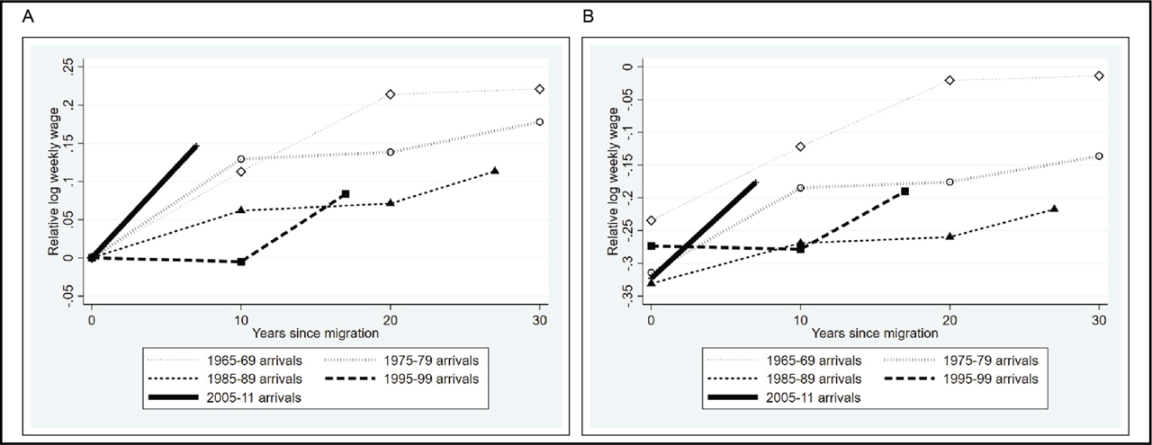
Figure 1
Age-adjusted convergences for the relative log weekly earnings of immigrant cohorts from all countries of origin: (A) normalized convergence; (B) initial gaps and convergence.
Notes: The wage differentials presented in this figure are calculated from regressions that are estimated separately for each cross section. The dependent variable in these regressions identifies the log weekly earnings of each individual, and the explanatory variables include a third-order polynomial for age and a set of fixed effects: one for each immigrant cohort. The omitted group comprises native-born workers such that the coefficients on the cohort fixed effects represent each cohort's log weekly earnings relative to that of native-born workers in a given survey year, which are used to construct the data points in the graphs. In Figure 1(A), the relative log weekly earnings for each cohort are normalized to zero at the time of entry.
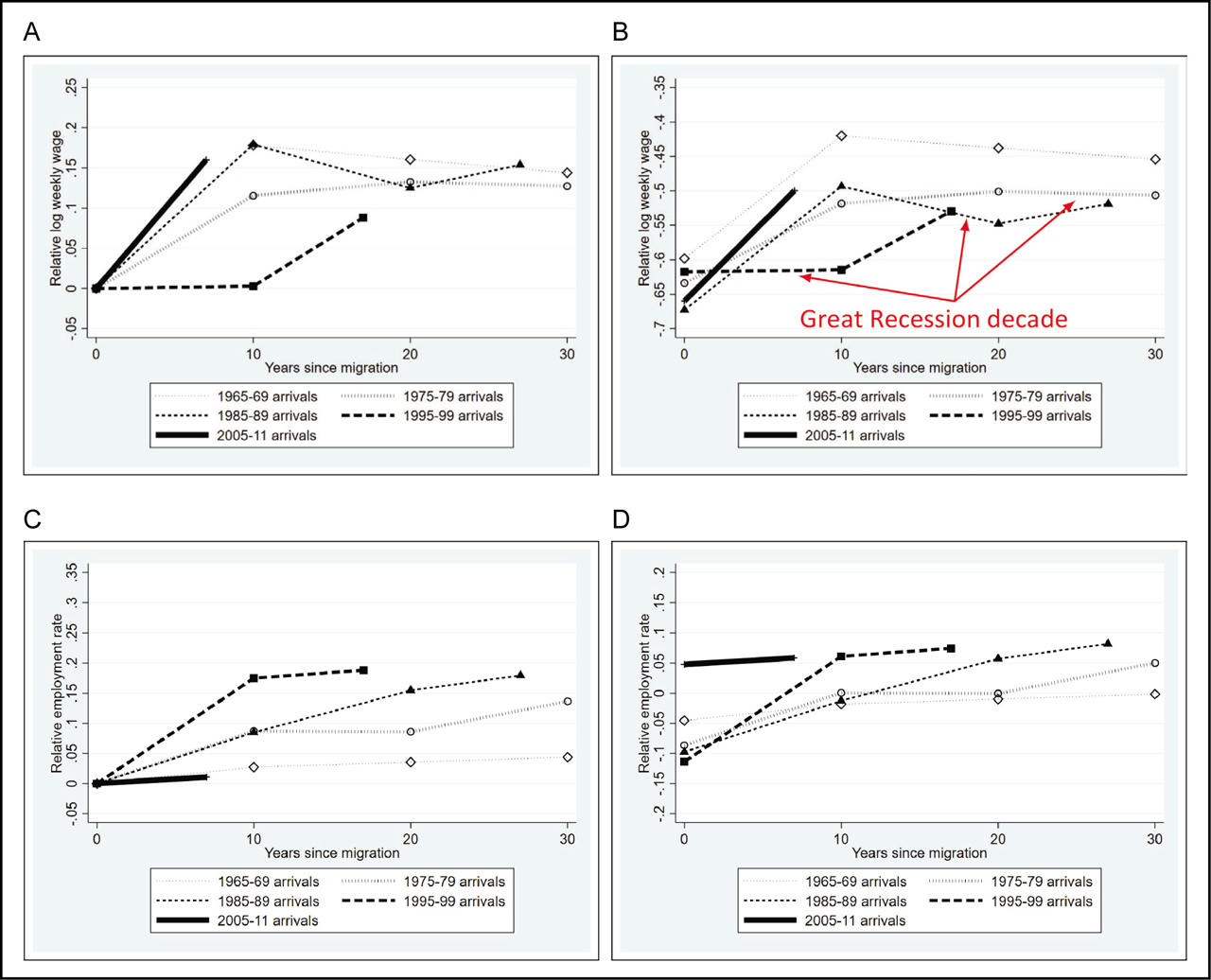
Figure 2
Age-adjusted convergences for the relative log weekly earnings and employment rates of Mexican and Central American immigrant cohorts: (A) normalized convergence; (B) initial gaps and convergence; (C) normalized convergence; (D) initial gaps and convergence.
Notes: The log weekly earnings and employment rate differentials presented in this figure are calculated from regressions that are estimated separately for each cross section. The dependent variable in the earnings regressions identifies the log weekly earnings of each individual. The dependent variable in the employment regressions identifies whether each individual was employed for at least 1 week during the previous year. The explanatory variables for both the earnings and the employment regressions include a third-order polynomial for age and a set of fixed effects: one for each immigrant cohort. The omitted group comprises native-born workers such that the coefficients on the cohort fixed effects represent each cohort's employment rate relative to that of native-born workers in a given survey year, which are used to construct the data points in the graphs. In Figure 2(A), the relative log weekly earnings for each cohort are normalized to zero at the time of entry. In Figure 2(C), the relative employment rate for each cohort is normalized to zero at the time of entry.
Table 1
Mexican and Central American immigrants: initial gaps and convergences after first 10 years
| (1) | (2) | |
|---|---|---|
| Panel A | ||
| Relative entry wage | ||
| 1965–1969 arrivals | −0.523** (0.044) | −0.449** (0.028) |
| 1975–1979 arrivals | −0.626** (0.042) | −0.437** (0.028) |
| 1985–1989 arrivals | −0.670** (0.046) | −0.445** (0.034) |
| 1995–1999 arrivals | −0.674** (0.023) | −0.423** (0.026) |
| 2005–2011 arrivals | −0.732** (0.016) | −0.427** (0.027) |
| 2012–17 arrivals | −0.530** (0.004) | −0.237** (0.026) |
| Panel B | ||
| Relative wage growth in first 10 years | ||
| 1965–1969 arrivals | 0.081 [0.202] | 0.221** [0.000] |
| 1975–1979 arrivals | 0.088 [0.162] | 0.216** [0.001] |
| 1985–1989 arrivals | 0.109 [0.102] | 0.198** [0.002] |
| 1995–1999 arrivals | 0.099* [0.031] | 0.181** [0.000] |
| 2005–2011 arrivals | 0.189 [0.000] | 0.239** [0.000] |
| Basic specification | X | – |
| Education–age–year FE | – | X |
| N | 9,669,594 | 9,669,594 |
Notes: The wage differentials presented in Panel A are generated from regressions that are run on the set of pooled cross sections from 1970, 1980, 1990, 2000, 2010, and 2017. The dependent variable identifies the log weekly earnings of each individual. The explanatory variables in Column 1 include a third-order polynomial for age, a third-order polynomial for the number of years that the immigrants have spent in the United States, a set of cohort fixed effects (FEs), and a set of cohort FEs that are each interacted with a continuous variable identifying the number of years that the immigrants have spent in the United States. The explanatory variables for Column 2 contain the same set of variables as in Column 1 but additionally include a set of education–age–year FEs. The omitted group comprises native-born workers such that the coefficients in Panel A each represent a separate cohort's log weekly earnings relative to native-born workers. The predicted relative wage growth in the first 10 years in Panel B assumes that all immigrants arrive in the country at the age of 25 years. Standard errors are in parentheses. P-values are in brackets.
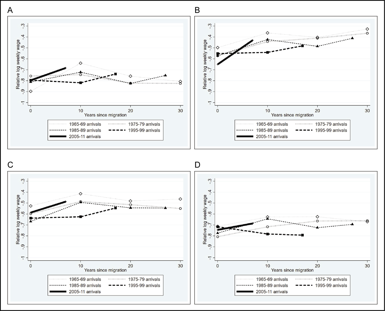
Figure 3
Age-adjusted convergences for the relative log weekly earnings of Mexican and Central American immigrant cohorts by sector: initial gaps and convergence. (A) agriculture and farming; (B) construction; (C) manufacturing; (D) personal and household services.
Notes: The wage differentials presented in this figure are calculated from regressions that are estimated separately for each cross section using data that only includes individuals employed in the sector identified in the panel being considered. The dependent variable in these regressions identifies the log weekly earnings of each individual, and the explanatory variables include a third-order polynomial for age and a set of fixed effects: one for each immigrant cohort. The omitted group comprises native-born workers such that the coefficients on the cohort fixed effects represent each cohort's log weekly earnings relative to native-born workers in a given survey year, which are used to construct the data points in the graphs.
Table 2
Mexican and Central American immigrants by sector: initial gaps and convergences after the first 10 years
| Agriculture | Construction | Manufacturing | Personal and household services | |||||
|---|---|---|---|---|---|---|---|---|
| (1) | (2) | (3) | (4) | (5) | (6) | (7) | (8) | |
| Panel A | ||||||||
| Relative entry wage | ||||||||
| 1965–1969 arrivals | −0.753** (0.033) | −0.606** (0.020) | −0.449** (0.047) | −0.339** (0.036) | −0.478** (0.032) | −0.409** (0.025) | −0.654** (0.037) | −0.570** (0.025) |
| 1975–1979 arrivals | −0.733** (0.034) | −0.500** (0.021) | −0.534** (0.041) | −0.325** (0.034) | −0.592** (0.031) | −0.393** (0.024) | −0.816** (0.036) | −0.612** (0.025) |
| 1985–1989 arrivals | −0.803** (0.036) | −0.490** (0.022) | −0.581** (0.041) | −0.337** (0.031) | −0.686** (0.038) | −0.448** (0.030) | −0.779** (0.036) | −0.536** (0.024) |
| 1995–1999 arrivals | −0.833** (0.020) | −0.489** (0.013) | −0.605** (0.020) | −0.317** (0.017) | −0.702** (0.017) | −0.423** (0.013) | −0.746** (0.018) | −0.481** (0.012) |
| 2005–2011 arrivals | −0.872** (0.014) | −0.461** (0.013) | −0.746** (0.014) | −0.368** (0.017) | −0.641** (0.015) | −0.289** (0.011) | −0.817** (0.013) | −0.459** (0.012) |
| 2012–17 arrivals | −0.860** (0.002) | −0.424** (0.008) | −0.562** (0.003) | −0.149** (0.013) | −0.506** (0.002) | −0.209** (0.003) | −0.609** (0.003) | −0.262** (0.007) |
| Panel B | ||||||||
| Relative wage growth in first 10 years | ||||||||
| 1965–1969 arrivals | 0.010 [0.854] | 0.147** [0.000] | 0.079 [0.161] | 0.207** [0.000] | 0.072 [0.162] | 0.243** [0.000] | 0.041 [0.457] | 0.184** [0.000] |
| 1975–1979 arrivals | −0.026 [0.618] | 0.114** [0.002] | 0.082 [0.122] | 0.209** [0.000] | 0.086† [0.093] | 0.237** [0.000] | 0.094† [0.093] | 0.224** [0.000] |
| 1985–1989 arrivals | 0.022 [0.679] | 0.117** [0.003] | 0.105† [0.060] | 0.197** [0.000] | 0.134** [0.021] | 0.253** [0.000] | 0.076 [0.166] | 0.169** [0.000] |
| 1995–1999 arrivals | 0.046 [0.245] | 0.129** [0.000] | 0.094* [0.016] | 0.176** [0.000] | 0.118** [0.003] | 0.227** [0.000] | 0.006 [0.862] | 0.099** [0.000] |
| 2005–2011 arrivals | 0.161** [0.000] | 0.201** [0.000] | 0.261** [0.000] | 0.313** [0.000] | 0.107** [0.000] | 0.165** [0.000] | 0.099** [0.000] | 0.120** [0.000] |
| N | 9,425,202 | 9,425,202 | 9,423,810 | 9,423,810 | 9,423,649 | 9,423,649 | 9,426,230 | 9,426,230 |
| Basic specification | X | – | X | – | X | – | X | – |
| Education–age–year FE | – | X | – | X | – | X | – | X |
Notes: The wage differentials presented in Panel A are generated from regressions that are run on the set of pooled cross sections from 1970, 1980, 1990, 2000, 2010, and 2017. The dependent variable identifies the log weekly earnings of each individual. The explanatory variables in Columns 1, 3, 5, and 7 include a third-order polynomial for age, a third-order polynomial for the number of years that the immigrants have spent in the United States, a set of cohort fixed effects (FEs), and a set of cohort FEs that are each interacted with a continuous variable identifying the number of years that the immigrants have spent in the United States. The explanatory variables for Columns 2, 4, 6, and 8 contain the same set of variables as in Column 1 but additionally include a set of education–age–year FEs. The omitted group is composed of native-born workers such that the coefficients in Panel A each represent a separate cohort's log weekly earnings relative to native-born workers. The predicted relative wage growth in the first 10 years in Panel B assumes that all immigrants arrive in the country at the age of 25 years. Standard errors are in parentheses. P-values are in brackets.
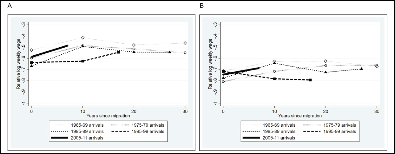
Figure 4
Age-adjusted convergences for the relative log weekly earnings of Mexican and Central American immigrant cohorts by location: initial gaps and convergences. (A) rural; (B) urban.
Notes: The wage differentials presented in this figure are calculated from regressions that are estimated separately for each cross section using data that only includes individuals employed in the region identified in the panel being considered. The dependent variable in these regressions identifies the log weekly earnings of each individual, and the explanatory variables include a third-order polynomial for age and a set of fixed effects: one for each immigrant cohort. The omitted group is composed of native-born workers such that the coefficients on the cohort fixed effects represent each cohort's log weekly earnings relative to native-born workers in a given survey year, which are used to construct the data points in the graphs.
Table 3
Mexican and Central American immigrants by location: initial gaps and convergences after first 10 years
| Rural | Urban | Enclave | Non-enclave | |||||
|---|---|---|---|---|---|---|---|---|
| (1) | (2) | (3) | (4) | (5) | (6) | (7) | (8) | |
| Panel A | ||||||||
| Relative entry wage | ||||||||
| 1965–1969 arrivals | −0.720** (0.0433) | −0.625** (0.0298) | −0.481** (0.0449) | −0.413** (0.0291) | −0.536** (0.054) | −0.448** (0.035) | −0.494** (0.024) | −0.452** (0.017) |
| 1975–1979 arrivals | −0.722** (0.0451) | −0.521** (0.0306) | −0.612** (0.0422) | −0.425** (0.0289) | −0.650** (0.043) | −0.450** (0.029) | −0.480** (0.040) | −0.362** (0.028) |
| 1985–1989 arrivals | −0.714** (0.0514) | −0.447** (0.0357) | −0.663** (0.0466) | −0.441** (0.0344) | −0.698** (0.048) | −0.461** (0.035) | −0.581** (0.041) | −0.379** (0.029) |
| 1995–1999 arrivals | −0.704** (0.0229) | −0.406** (0.0169) | −0.668** (0.228) | −0.419** (0.0249) | −0.705** (0.025) | −0.445** (0.023) | −0.629** (0.017) | −0.369** (0.015) |
| 2005–2011 arrivals | −0.647** (0.0152) | −0.320** (0.0124) | −0.743** (0.0163) | −0.434** (0.0255) | −0.751** (0.017) | −0.434** (0.019) | −0.711** (0.012) | −0.393** (0.019) |
| 2012–17 arrivals | −0.512** (0.00284) | −0.147** (0.00513) | −0.531** (0.00363) | −0.243** (0.0236) | −0.570** (0.003) | −0.270** (0.015) | −0.484** (0.002) | −0.176** (0.018) |
| N | 9,112,492 | 9,112,492 | 9,331,676 | 9,331,676 | 9,588,212 | 9,588,212 | 9,465,090 | 9,465,090 |
| Panel B | ||||||||
| Relative wage growth in first 10 years | ||||||||
| 1965–1969 arrivals | 0.047 [0.476] | 0.207** [0.000] | 0.073 [0.257] | 0.213** [0.000] | 0.086 [0.224] | 0.226** [0.000] | 0.096† [0.057] | 0.208** [0.000] |
| 1975–1979 arrivals | 0.093 [0.188] | 0.232** [0.000] | 0.084 [0.183] | 0.212** [0.000] | 0.103 [0.124] | 0.228** [0.000] | 0.024 [0.653] | 0.167** [0.000] |
| 1985–1989 arrivals | 0.097 [0.184] | 0.193** [0.001] | 0.107 [0.110] | 0.197** [0.000] | 0.126† [0.077] | 0.211** [0.000] | 0.056 [0.304] | 0.161** [0.001] |
| 1995–1999 arrivals | 0.079 [0.092] | 0.171** [0.000] | 0.098* [0.034] | 0.180** [0.000] | 0.119* [0.019] | 0.202** [0.000] | 0.062† [0.075] | 0.147** [0.000] |
| 2005–2011 arrivals | 0.067 [0.001] | 0.170** [0.000] | 0.204** [0.000] | 0.249** [0.000] | 0.195** [0.000] | 0.240** [0.000] | 0.182** [0.000] | 0.242** [0.000] |
| Basic specification | X | – | X | – | X | – | X | – |
| Education–age–year FE | – | X | – | X | – | X | – | X |
Notes: The wage differentials presented in Panel A are generated from regressions that are run on the set of pooled cross sections from 1970, 1980, 1990, 2000, 2010, and 2017. The dependent variable identifies the log weekly earnings of each individual. The explanatory variables in Columns 1, 3, 5, and 7 include a third-order polynomial for age, a third-order polynomial for the number of years that the immigrants have spent in the United States, a set of cohort fixed effects (FEs), and a set of cohort FEs that are each interacted with a continuous variable identifying the number of years that the immigrants have spent in the United States. The explanatory variables for Columns 2, 4, 6, and 8 contain the same set of variables as in Column 1 but additionally include a set of education–age–year FEs. The omitted group is composed of native-born workers such that the coefficients in Panel A each represent a separate cohort's log weekly earnings relative to native-born workers. The predicted relative wage growth in the first 10 years in Panel B assumes that all immigrants arrive in the country at the age of 25 years. The enclave states are the states with the largest percentage of Mexican and Central Americans in the population over the period 1970–2017. They include California, Texas, Arizona, New Mexico, Nevada, and Illinois. Standard errors are in parentheses. P-values are in brackets.
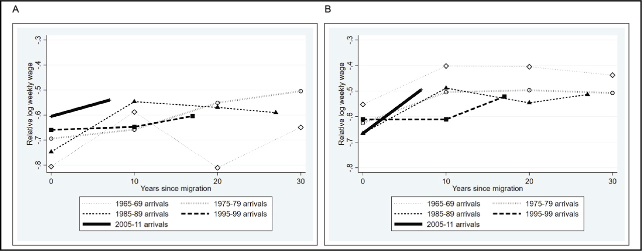
Figure 5
Age-adjusted convergences for the relative log weekly earnings of Mexican and Central American immigrant cohorts by enclave region: initial gaps and convergences. (A) enclave; (B) non-enclave.
Notes: The wage differentials presented in this figure are calculated from regressions that are estimated separately for each cross section using data that only includes individuals employed in the region identified in the panel being considered. The dependent variable in these regressions identifies the log weekly earnings of each individual, and the explanatory variables include a third-order polynomial for age and a set of fixed effects: one for each immigrant cohort. The omitted group is composed of native-born workers such that the coefficients on the cohort fixed effects represent each cohort's log weekly earnings relative to native-born workers in a given survey year, which are used to construct the data points in the graphs. The enclave states are the states with the largest percentage of Mexican and Central Americans in the population over the period 1970–2017. They include California, Texas, Arizona, New Mexico, Nevada, and Illinois.
Table 4
Summary statistics for Mexican and Central American immigrant cohorts upon arrival
| Cohort | 1965–69 | 1975–79 | 1985–89 | 1995–99 | 2005–11 |
|---|---|---|---|---|---|
| Age | 34.24 | 33.11 | 32.85 | 32.98 | 33.73 |
| Years of schooling | 6.79 | 6.79 | 7.29 | 7.79 | 8.29 |
| Share of Central Americans | 0.18 | 0.14 | 0.26 | 0.15 | 0.29 |
| Share of those speaking some English | No data | 0.66 | 0.69 | 0.65 | 0.67 |
| Share of those speaking good English | No data | 0.28 | 0.31 | 0.29 | 0.27 |
| Share of nonwhites | 0.06 | 0.06 | 0.56 | 0.55 | 0.42 |
| Share of noncitizens at arrival | 0.78 | 0.89 | 0.92 | 0.95 | 0.97 |
Table A1
Age-adjusted relative log weekly earnings of immigrant cohorts from all countries of origin by census cross section
| Cohort | 1970 | 1980 | 1990 | 2000 | 2010 | 2017 |
|---|---|---|---|---|---|---|
| 1950–59 arrivals | 0.037** (0.000) | 0.032** (0.002) | 0.100** (0.003) | 0.147** (0.010) | . . . | . . . |
| 1960–64 arrivals | −0.058** (0.001) | −0.041** (0.001) | 0.046** (0.004) | 0.074** (0.004) | 0.594** (0.019) | . . . |
| 1965–1969 arrivals | −0.235** (0.001) | −0.122** (0.000) | −0.020** (0.003) | −0.014* (0.005) | 0.196** (0.010) | . . . |
| 1970–74 arrivals | . . . | −0.223** (0.001) | −0.124** (0.002) | −0.128** (0.006) | −0.057** (0.004) | 0.161** (0.012) |
| 1975–1979 arrivals | . . . | −0.314** (0.001) | −0.185** (0.000) | −0.176** (0.005) | −0.136** (0.004) | −0.118** (0.007) |
| 1980–84 arrivals | . . . | . . . | −0.285** (0.001) | −0.236** (0.002) | −0.206** (0.006) | −0.188** (0.010) |
| 1985–1989 arrivals | . . . | . . . | −0.331** (0.001) | −0.269** (0.002) | −0.260** (0.005) | −0.218** (0.011) |
| 1990–94 arrivals | . . . | . . . | . . . | −0.269** (0.003) | −0.271** (0.003) | −0.168** (0.010) |
| 1995–1999 arrivals | . . . | . . . | . . . | −0.273** (0.004) | −0.279** (0.001) | −0.190** (0.006) |
| 2000–04 arrivals | . . . | . . . | . . . | . . . | −0.349** (0.003) | −0.224** (0.003) |
| 2005–2011 arrivals | . . . | . . . | . . . | . . . | −0.323** (0.004) | −0.176** (0.003) |
| 2012–17 arrivals | . . . | . . . | . . . | . . . | . . . | −0.103** (0.005) |
| N | 945,579 | 2,002,074 | 2,373,285 | 2,708,438 | 1,653,425 | 557,077 |
Note: The wage dierentials presented in this table are calculated from regressions that are estimated separately for each cross section, which are identied by the year displayed in the column heading. The dependent variable identies the log weekly earnings of each individual, and the explanatory variables include a third-order polynomial for the age of the individual and a set of xed eects: one for each immigrant cohort, including one (not shown in the table) for the cohort that arrived in the US prior to 1950. The omitted group is comprised of native-born workers such that the coecients in a column each represent a separate cohort's log weekly earnings relative to native-born workers in that survey year. The \2010" cross section is generated from the pooled 2009–11 American Community Surveys. Standard errors in parentheses are clustered at the cohort level.
Table A2
Population Estimates for Mexican and Central American Immigrant Cohorts
| Cohort | Survey Year | |||||
|---|---|---|---|---|---|---|
| 1970 | 1980 | 1990 | 2000 | 2010 | 2017 | |
| 1965–1969 arrivals | 39,467 | 81,060 | 72,985 | 59,455 | 2,736 | . . . |
| 1975–1979 arrivals | . . . | 147,640 | 240,400 | 267,721 | 149,135 | 38,555 |
| 1985–1989 arrivals | . . . | . . . | 286,304 | 631,788 | 486,691 | 369,182 |
| 1995–1999 arrivals | . . . | . . . | . . . | 640,099 | 768,334 | 653,910 |
| 2005–2011 arrivals | . . . | . . . | . . . | . . . | 595,641 | 682,617 |
| Natives | 34,734,070 | 40,998,200 | 47,947,840 | 53,784,860 | 57,155,860 | 61,335,820 |
[i] Note: These gures estimate the population of native-born and Mexican and Central American immigrant males between the ages of 25 and 64 who had between 1 and 40 years of potential work experience, were not in school or living in group quarters, and (for immigrants) entered the US at the age of 18 or older.
Table A3
Percentage of workforce composed of Mexican and Central American immigrants by sector and location
| Survey year | ||||||
|---|---|---|---|---|---|---|
| 1970 | 1980 | 1990 | 2000 | 2010 | 2017 | |
| Panel A: by sector | ||||||
| Agriculture and farming | 1.5 | 4.7 | 10.5 | 19.6 | 27.8 | 23.8 |
| Construction | 0.4 | 1.1 | 2.8 | 7.5 | 13.1 | 15.1 |
| Manufacturing | 0.8 | 2.7 | 4.4 | 8.5 | 9.7 | 7.5 |
| Personal and household services | 0.7 | 2.1 | 4.3 | 7.5 | 9.3 | 7.2 |
| All sectors | 0.4 | 1.1 | 2.1 | 4.4 | 6 | 5.4 |
| Panel B: by location | ||||||
| Rural | 0.2 | 0.4 | 0.6 | 1.8 | 2.8 | 2.5 |
| Urban | 0.5 | 1.5 | 2.8 | 5.2 | 6.9 | 6.1 |
| Enclave | 1.6 | 4.2 | 6.9 | 11.7 | 13.3 | 11.5 |
| Nonenclave | 0.2 | 0.2 | 0.5 | 1.8 | 3.3 | 3.1 |
[i] Notes: These figures only include US-born, Mexican, and Central American males between the ages of 25 and 64 years who had between 1 years and 40 years of potential work experience, were not in school or living in group quarters, had positive earnings, worked at least 1 week during the survey year, and (for immigrants) entered the United States at the age of 18 years or older. The enclave states used here are based on the share of Mexican and Central American immigrants calculated over the time period 1970–2017. They include California, Texas, Arizona, New Mexico, Nevada, and Illinois.
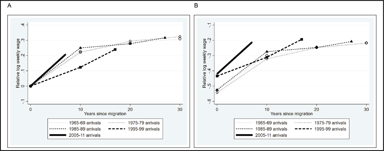
Figure A1
Age-adjusted convergences for the relative weekly earnings of Mexican and Central American immigrant cohorts, only high school educated or less: (A) normalized convergence; (B) initial gap and convergence.
Notes: The wage differentials presented in this figure are calculated from regressions that are estimated separately for each cross section. The dependent variable in these regressions identifies the log weekly earnings of each individual, and the explanatory variables include a third-order polynomial for age and a set of fixed effects: one for each immigrant cohort. The omitted group is composed of native-born workers such that the coefficients on the cohort fixed effects represent each cohort's log weekly earnings relative to native-born workers in a given survey year, which are used to construct the data points in the graphs. In Figure A1a, the relative log weekly earnings for each cohort are normalized to zero at the time of entry. In Figure A1a and A1b, all individuals (both natives and immigrants) have had a high school education or less.