
Figure 1
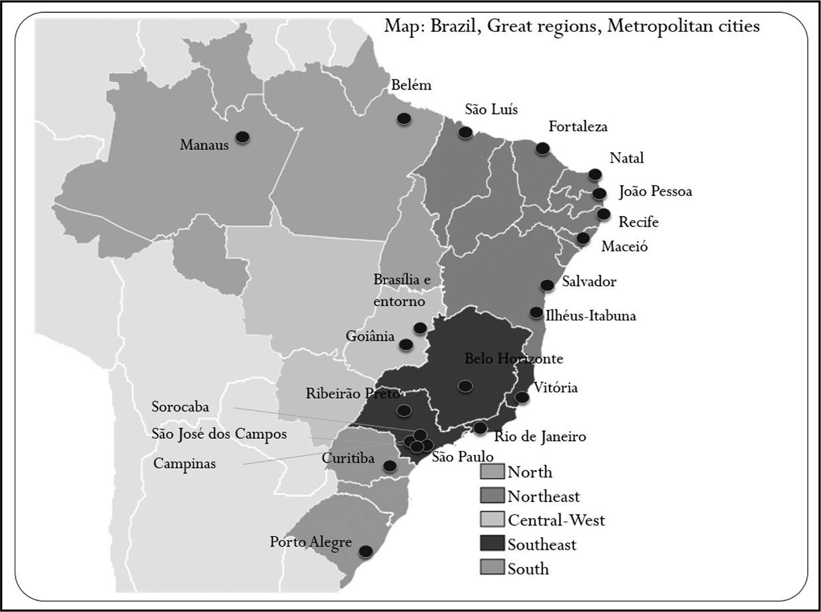
Figure 2
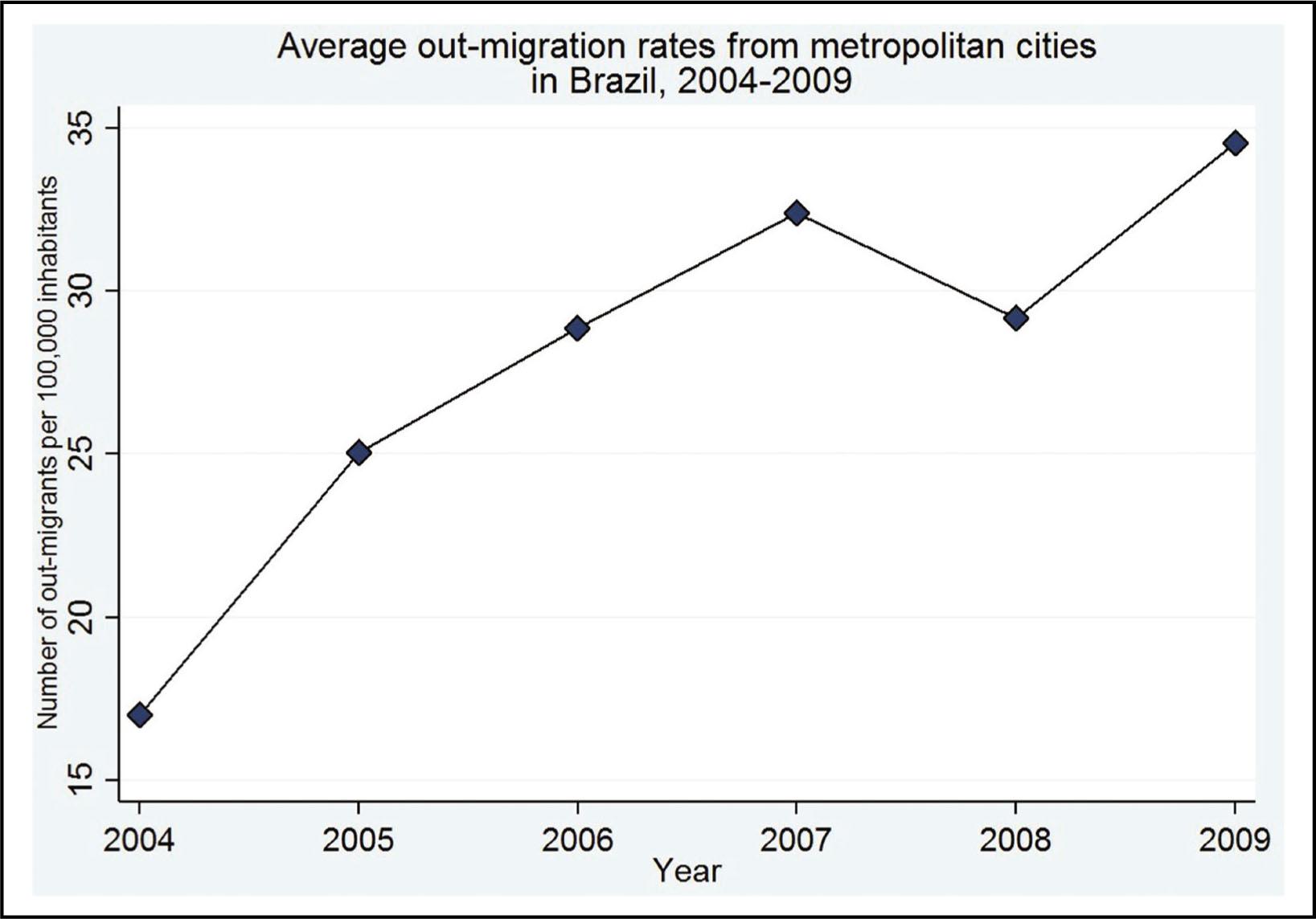
Figure 3
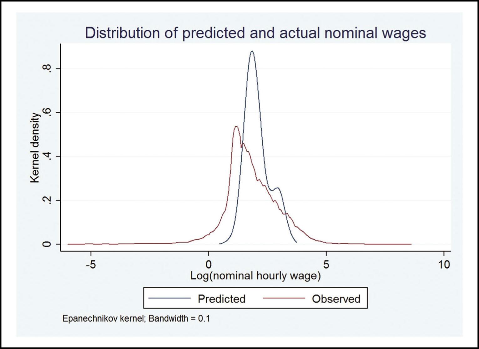
Figure 4
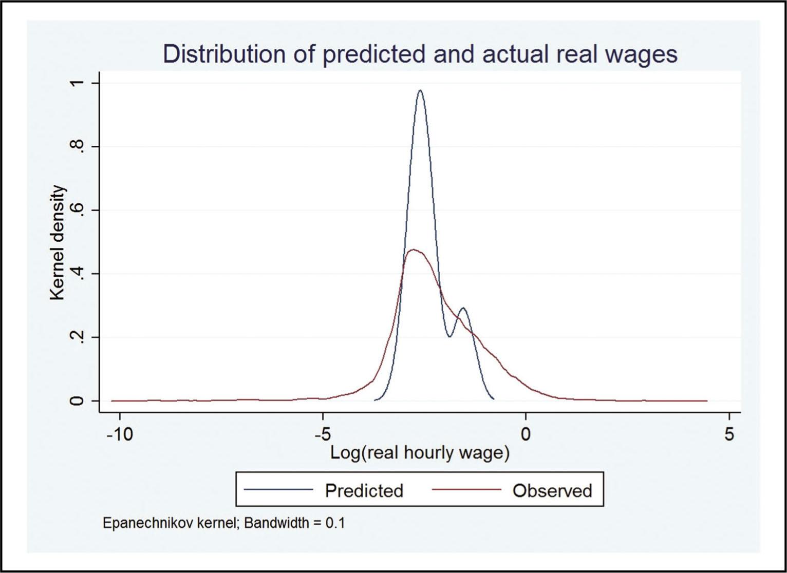
Figure A1
Balancing statistics after matching
| Multivariate L1 distance: | 0.78689126 | ||||||
|---|---|---|---|---|---|---|---|
| Univariate imbalance: | L1 | Mean | Min | 25% | 50% | 75% | Max |
| Age at migration | 0.04019 | −0.15014 | 0 | 0 | 0 | −1 | 0 |
| Sex | 0.06926 | −0.06926 | 0 | 0 | 0 | 0 | 0 |
| Education level | 0.03117 | −0.03117 | 0 | 0 | 0 | 0 | 0 |
| Race | 0.00467 | −0.00467 | 0 | 0 | 0 | 0 | 0 |
| City of origin | 0.00479 | 0.00479 | 0 | 0 | 0 | 0 | 0 |
| Marital status | 0.02571 | −0.02571 | 0 | 0 | 0 | 0 | 0 |
| Sector of activity | 0.00355 | 0.00355 | 0 | 0 | 0 | 0 | 0 |
Migrants between metropolitan and non-metropolitan microregiões between 2009 and 2010
| Destination | ||||
|---|---|---|---|---|
| Non-metropolitan | Metropolitan | |||
| Origin | N | % | N | % |
| Non-metropolitan | 380,627 | 46.9 | 167,781 | 20.7 |
| Metropolitan | 162,647 | 20.1 | 99,143 | 12.2 |
Labor market characteristics of migrants and non-migrants 2010
| Non-metropolitan residents | Metropolitan out-migrants | Metropolitan residents | |
|---|---|---|---|
| Unemployed | 0.05 | 0.12 | 0.06 |
| Log (monthly wages) | 6.59 | 6.95 | 6.98 |
| Sector | |||
| Formal private | 0.40 | 0.43 | 0.56 |
| Formal public | 0.06 | 0.08 | 0.06 |
| Informal | 0.26 | 0.23 | 0.21 |
| Self-employed | 0.02 | 0.02 | 0.01 |
| Small business | 0.26 | 0.24 | 0.15 |
| Industry, ISIC | |||
| Agriculture | 0.26 | 0.14 | 0.09 |
| Industry | 0.22 | 0.27 | 0.21 |
| Services | 0.38 | 0.44 | 0.54 |
| Public services | 0.15 | 0.17 | 0.17 |
Destination choice conditional on migration, alternative specific logit
| (1) | (2) | (3) | |
|---|---|---|---|
| Wage measure: | Expected wages (log) | Matched expected wages (log) | |
| Price measure: | Rent per room (log) | Wages in neighboring locations (log) | |
| Difference in: | |||
| Wages | 0.054 (0.175) | −0.041 (0.234) | −0.069 (0.244) |
| Prices | −0.173 (0.213) | −0.805 (0.730) | −0.822 (0.631) |
| Population (log) | −0.019 (0.068) | −0.040 (0.064) | 0.011 (0.080) |
| Homicide rate | 0.004 (0.004) | ||
| Health facilities | 0.008*** (0.003) | ||
| Health quality index | −1.292* (0.758) | ||
| Education quality index | 1.569* (0.929) | ||
| Destination specific: | |||
| Distance to origin (log) | −0.524*** (0.085) | −0.523*** (0.087) | −0.521*** (0.087) |
| Other state | −1.800*** (0.265) | −1.850*** (0.258) | −1.853*** (0.250) |
| Observations | 5730782 | 5730782 | 5730782 |
| Wald chi2 | 742 | 1222 | 1367 |
| Number of cases | 14509 | 14509 | 14509 |
| Number of alternatives | 514 | 514 | 514 |
Differences in actual and predicted wages for metropolitan out-migrants, by education level
| High-educated | ||
| Log (nominal hourly wages) | N | Mean |
| Observed | 3,107 | 2.846 |
| Predicted | 3,107 | 2.930 |
| Difference | −0.084*** | |
| Log (real hourly wages) | N | Mean |
| Observed | 3,107 | −1.270 |
| Predicted | 3,107 | −1.544 |
| Difference | 0.274*** | |
| Low-educated | ||
| Log (nominal hourly wages) | N | Mean |
| Observed | 12,317 | 1.556 |
| Predicted | 12,317 | 1.851 |
| Difference | −0.295*** | |
| Log (real hourly wages) | N | Mean |
| Observed | 12,317 | −2.481 |
| Predicted | 12,317 | −2.611 |
| Difference | 0.130*** | |
Differences of actual and predicted wages for metropolitan out-migrants, before matching
| Log (nominal hourly wages) | N | Mean |
| Observed | 14,810 | 1.767 |
| Predicted | 14,810 | 1.874 |
| Difference | −0.107*** | |
| Log (real hourly wages) | N | Mean |
| Observed | 14,810 | −2.466 |
| Predicted | 14,810 | 0.303 |
| Difference | 0.303*** | |
| Log (real hourly wages) | N | Mean |
| Hedonic price as denominator | ||
| Observed | 14,810 | −2.353 |
| Predicted | 14,810 | 0.204 |
| Difference | 0.204*** | |
Matching summary
| Number of strata: | 9,796 | |
|---|---|---|
| Number of matched strata: | 3,785 | |
| Non-migrants | Migrants | |
| All | 683,517 | 16,172 |
| Matched | 587,346 | 15,401 |
| Unmatched | 96,171 | 771 |
Differences in actual and predicted real wages for metropolitan out-migrants using hedonic prices as a denominator, after matching
| Log (real hourly wages) | N | Mean |
|---|---|---|
| Observed | 15,424 | −2.105 |
| Predicted | 15,424 | −2.155 |
| Difference | 0.050*** |
Observed and predicted real wage differences using different measures of living costs, metropolitan in-migrants
| Log (real hourly wages) | ||
|---|---|---|
| High skilled | ||
| Skill-specific mean rents | N | Mean |
| Observed | 1,068 | −1.931 |
| Predicted | 1,068 | −1.974 |
| Difference | 0.043* | |
| Skill-specific median rents | N | Mean |
| Observed | 1,068 | −1.795 |
| Predicted | 1,068 | −1.894 |
| Difference | 0.099*** | |
| Low skilled | ||
| Skill-specific mean rents | N | Mean |
| Observed | 7,357 | −2.775 |
| Predicted | 7,357 | −2.501 |
| Difference | −0.274*** | |
| Skill-specific median rents | N | Mean |
| Observed | 7,357 | −2.680 |
| Predicted | 7,357 | −2.394 |
| Difference | −0.286*** | |
Difference between non-metropolitan destination and metropolitan origin comparing chosen destination to alternative destinations
| Difference between destination and origin in | Chosen destination | Alternative destinations | t-statistic, difference in mean |
|---|---|---|---|
| Expected hourly wages (log) | −0.53 | −0.61 | −24.7 |
| Matched expected wages (log) | −2.73 | −2.79 | −16.2 |
| Rent per room (log) | −0.55 | −0.64 | −21.9 |
| IV (wages in neighboring MRs, log) | −0.10 | −0.14 | −23.5 |
| Population in thousands | −5,605 | −6,326 | −17.1 |
| Homicide rate | −17.66 | −14.11 | 18.2 |
| Health facilities (per 100,000) | 25.49 | 26.46 | 8.1 |
| Health provision quality index (0–1) | −0.03 | −0.05 | −24.0 |
| Education provision quality index (0–1) | −0.00 | −0.04 | −32.8 |
| Distance to origin (km) | 573 | 1,295 | 108.6 |
| Other state than origin | 0.45 | 0.92 | 202.4 |
Regression of housing prices on housing characteristics, OLS estimates
| log(rent per room) | |
|---|---|
| Urban area | 0.256*** (0.005) |
| Type of dwelling (Base = House) | |
| Townhouse/condominion | 0.146*** (0.003) |
| Flat | 0.396*** (0.002) |
| Hut | 0.196*** (0.006) |
| Wall material (Base = Bricks coated) | |
| Bricks not coated | −0.160*** (0.002) |
| Wood | −0.265*** (0.003) |
| Plaster coated | −0.461*** (0.015) |
| Plaster not coated | −0.521*** (0.020) |
| Wood unprepared | −0.344*** (0.010) |
| Straw | −0.073 (0.155) |
| Others | −0.146*** (0.015) |
| Bathroom (Base = none) | |
| 1 | −0.213*** (0.006) |
| 2 | −0.095*** (0.006) |
| 3 | 0.047*** (0.007) |
| 4 | 0.220*** (0.012) |
| 5 | 0.355*** (0.027) |
| 6 | 0.517*** (0.054) |
| 7 | 0.430*** (0.119) |
| 8 | 1.046*** (0.237) |
| 9 or more | 0.356*** (0.083) |
| Sanitation (Base = General sanitation network) | |
| Septic sump | −0.089*** (0.002) |
| Rudimentary Sump | −0.200*** (0.002) |
| Ditch | −0.225*** (0.005) |
| River, lake or sea | −0.152*** (0.004) |
| Other | −0.212*** (0.009) |
| Waste water (Base = General distribution network) | |
| Well on property | 0.007** (0.003) |
| Well outside property | −0.088*** (0.005) |
| Carro-pipa | −0.072*** (0.014) |
| Rainwater cistern | −0.074*** (0.028) |
| Rain water other | −0.097 (0.068) |
| Rivers, lakes, etc. | −0.081*** (0.023) |
| Other | −0.155*** (0.010) |
| Well in village | 0.165** (0.066) |
| Canalization access (Base = Yes, in min. 1 room) | |
| Yes, only on the property | −0.052*** (0.004) |
| No | −0.148*** (0.006) |
| Garbage collection (Base = Collected directly) | |
| Collected in collective | −0.054*** (0.002) |
| Burnt | −0.229*** (0.008) |
| Buried | −0.017 (0.043) |
| Tossed in a public area | −0.229*** (0.008) |
| Tossed in river, lake, or sea | −0.195*** (0.036) |
| Other | 0.005 (0.027) |
| Electricity provision (base = Yes by the company) | |
| Yes, other | −0.094*** (0.010) |
| No electricity | −0.238*** (0.021) |
| Constant | 4.235*** (0.016) |
| Microregion dummies | Yes |
| Observations | 927,192 |
| R-squared | 0.539 |
Characteristics of metropolitan and non-metropolitan microregiões in 2010
| Metropolitan | Non-metropolitan | |||
|---|---|---|---|---|
| Mean | Coeff. of variation | Mean | Coeff. of variation | |
| Population | 2,679,687 | 1.11 | 213,680 | 0.79 |
| Room rent (R$, median) | 72.47 | 0.23 | 45.22 | 0.42 |
| Hourly wage (R$) | 12.11 | 0.22 | 7.23 | 0.29 |
| Share of | ||||
| Unskilled workers | 0.37 | 0.09 | 0.37 | 0.14 |
| Skilled workers | 0.31 | 0.11 | 0.40 | 0.14 |
| High-skilled workers | 0.24 | 0.17 | 0.16 | 0.23 |
| Formally employed | 0.58 | 0.11 | 0.40 | 0.36 |
| Unemployed | 0.06 | 0.29 | 0.05 | 0.41 |
| Share of workers in | ||||
| Agriculture | 0.09 | 0.36 | 0.30 | 0.39 |
| Industry | 0.21 | 0.23 | 0.18 | 0.37 |
| Services | 0.53 | 0.08 | 0.35 | 0.23 |
| Public services | 0.11 | 0.25 | 0.12 | 0.24 |
| People living in | ||||
| Adequate living conditions | 0.57 | 0.28 | 0.36 | 0.67 |
| Other measures | ||||
| GDP growth 2005–2010 | 0.16 | 0.31 | 0.18 | 0.79 |
| Health facilities (per 100,000) | 16.40 | 0.42 | 41.86 | 0.35 |
| Health quality index (0–1) | 0.82 | 0.09 | 0.79 | 0.11 |
| Education quality index (0–1) | 0.77 | 0.14 | 0.73 | 0.14 |
| Homicide rate (per 100,000) | 38.00 | 0.54 | 18.58 | 0.77 |
Differences in actual and predicted wages for metropolitan out-migrants, after matching
| Log (nominal hourly wages) | N | Mean |
| Observed | 15,424 | 1.816 |
| Predicted | 15,424 | 2.069 |
| Difference | −0.253*** | |
| Log (real hourly wages) | N | Mean |
| Observed | 15,424 | −2.237 |
| Predicted | 15,424 | −2.396 |
| Difference | 0.159*** | |
Observed and predicted real wage differences using different measures of living costs
| Log (real hourly wages) | ||
|---|---|---|
| Low skilled | ||
| Skill-specific mean rents | N | Mean |
| Observed | 11,393 | −2.456 |
| Predicted | 11,393 | −2.691 |
| Difference | 0.235*** | |
| Skill-specific median rents | N | Mean |
| Observed | 11,393 | −2.365 |
| Predicted | 11,393 | −2.589 |
| Difference | 0.224*** | |
| Median hedonic prices | N | Mean |
| Observed | 11,393 | −2.374 |
| Predicted | 11,393 | −2.555 |
| Difference | 0.181*** | |
Balancing statistics before matching
| Multivariate L1 distance: | 0.83541258 | ||||||
|---|---|---|---|---|---|---|---|
| Univariate imbalance: | L1 | Mean | Min | 25% | 50% | 75% | Max |
| Age at migration | 0.10634 | −2.2895 | −1 | −1 | −3 | −3 | −1 |
| Sex | 0.0979 | −0.0979 | 0 | 0 | 0 | 0 | 0 |
| Education level | 0.07352 | −0.12922 | 0 | −1 | 0 | 0 | 0 |
| Race | 0.00576 | 0.00576 | 0 | 0 | 0 | 0 | 0 |
| City of origin | 0.14503 | 0.72656 | 0 | 0 | 4 | 0 | 0 |
| Marital status | 0.01909 | −0.0098 | 0 | 0 | 0 | 0 | 0 |
| Sector of activity | 0.15388 | −0.96689 | 0 | −3 | −1 | 0 | −1 |
Destination choice conditional on migration by the education of migrant, alternative specific logit
| (1) | (2) | (3) | (4) | |
|---|---|---|---|---|
| Level of education: | None or primary | Lower secondary | Upper secondary | Higher |
| Difference in: | ||||
| Matched expected wages (log) | −0.279 (0.255) | −0.161 (0.328) | −0.023 (0.238) | 0.336 (0.238) |
| Prices (IV) | −1.360* (0.700) | −1.205* (0.691) | −0.686 (0.638) | 0.202 (0.563) |
| Population (log) | −0.028 (0.093) | 0.049 (0.112) | 0.022 (0.076) | 0.036 (0.069) |
| Homicide rate | 0.004 (0.004) | 0.003 (0.003) | 0.006 (0.004) | 0.000 (0.004) |
| Health facilities | 0.009*** (0.004) | 0.010** (0.004) | 0.008** (0.003) | 0.002 (0.003) |
| Health quality index | −0.787 (0.950) | −0.754 (0.953) | −1.668* (0.886) | −2.184** (0.852) |
| Education quality index | 1.684 (1.128) | 1.238 (1.114) | 1.977* (1.019) | 1.055 (0.693) |
| Destination specific: | ||||
| Distance to origin (log) | −0.496*** (0.086) | −0.574*** (0.081) | −0.515*** (0.102) | −0.538*** (0.104) |
| Other state | −1.963*** (0.253) | −1.808*** (0.261) | −1.881*** (0.281) | −1.663*** (0.282) |
| Observations | 1871193 | 954109 | 1840023 | 1065457 |
| Wald chi2 | 765 | 1255 | 1658 | 2850 |
| Number of cases | 4835 | 2425 | 4598 | 2651 |
| Number of alternatives | 514 | 514 | 514 | 514 |
Elasticities of significant covariates by sub-sample
| Education | No or primary | Lower secondary | Upper secondary | Higher |
|---|---|---|---|---|
| Distance (log) | −3.4 | −4.0 | −3.6 | −3.7 |
| Other state | −1.8 | −1.7 | −1.7 | −1.5 |
| Health facilities | 0.2 | 0.3 | 0.2 | 0.1 |
| Prices (IV) | 0.2 | 0.2 | 0.1 | 0.0 |
| Education quality | −0.1 | −0.1 | −0.1 | 0.0 |
| Health quality | 0.0 | 0.0 | 0.1 | 0.1 |
Coefficients and t-statistics of prediction of wages for migrants based on past migrants at the destination, OLS
| Log(hourly wage) | ||
|---|---|---|
| Coefficient | t-statistic | |
| Age | 0.048 | 18.250 |
| Age squared | −0.045 | −13.939 |
| Female | −0.368 | −61.567 |
| White | 0.123 | 19.385 |
| Education (Base = none) | ||
| Primary, secondary incomplete | 0.240 | 28.118 |
| Secondary, higher incomplete | 0.530 | 71.485 |
| Higher complete | 1.441 | 154.831 |
| Mean (Log (hourly wage)) = | −0.754 | |
Characteristics of migrants and non-migrants 2010
| Non-metropolitan residents | Metropolitan out-migrants | Metropolitan residents | |
|---|---|---|---|
| Number of observations | 4,184,904 | 19,318 | 1,598,869 |
| Age | 40.25 | 36.85 | 40.22 |
| Female | 0.41 | 0.37 | 0.45 |
| White | 0.51 | 0.51 | 0.51 |
| Education level | |||
| None, primary incomplete | 0.47 | 0.29 | 0.29 |
| Primary, secondary incomplete | 0.16 | 0.16 | 0.17 |
| Secondary, higher incomplete | 0.26 | 0.33 | 0.36 |
| Higher complete | 0.11 | 0.21 | 0.19 |
Variables and data sources
| Variable | Description | Source |
|---|---|---|
| Variables for descriptive statistics and destination choice model on microregião level | ||
| Wages (IV) | Average monthly wages in neighboring microregião | RAIS* |
| Housing prices | Average rent on microregião level | Census, IBGE |
| Education provision quality index | Index from 0 to 1, computed based on: Subscription rate of pre-school children, dropout rate | FIRJAN** |
| Rate of teachers with higher education, average daily teaching hours, results of the IDEB (Indicator of development of education in Brazil) | ||
| Health provision quality index | Index from 0 to 1, computed based on: Number of pre-natal consultations, deaths due to mal-defined causes, child-deaths due to evitable causes | FIRJAN** |
| Number of health care facilities | Per 100,000 inhabitants; include general hospitals, day hospitals, polyclinics, health point, general emergency, pharmacy, basic health center. | CNES*** |
| Homicide rate | Per 100,000 inhabitants in 2008 | Ipeadata |
| Distance to the state capital | Indicator for market access (Fally et al. 2010) | Ipeadata |
| GDP | Log of GDP in 2009 | Ipeadata |
| Distance between origin and destination | Geodesic distance as an indicator for fixed moving costs, author's calculation from coordinates | Census, IBGE |
| Additional variables for wage regression, on an individual level | ||
| Partner participation | Dummy whether the partner is working | Census, IBGE |
| The proportion of children in the household | Census, IBGE | |
| Marital status | Separated/divorced/widowed, single, married | Census, IBGE |
| Sector | Public, private, informal, self-employed | Census, IBGE |
| Industry | 21 industries according to International Standard Industrial Classification of all Economic Activities (ISIC) | Census, IBGE |
| Federal state | 27 states | Census, IBGE |
| Variables for matching, on an individual level | ||
| Age | At the time of migration, i.e., one year ago | Census, IBGE |
| Race | White and non-white | Census, IBGE |
| Education level | Primary, middle, high-school, college | Census, IBGE |
| Micro-region of origin/residency | City of origin for migrants and city of residency for comparison group of non-migrants | Census, IBGE |