
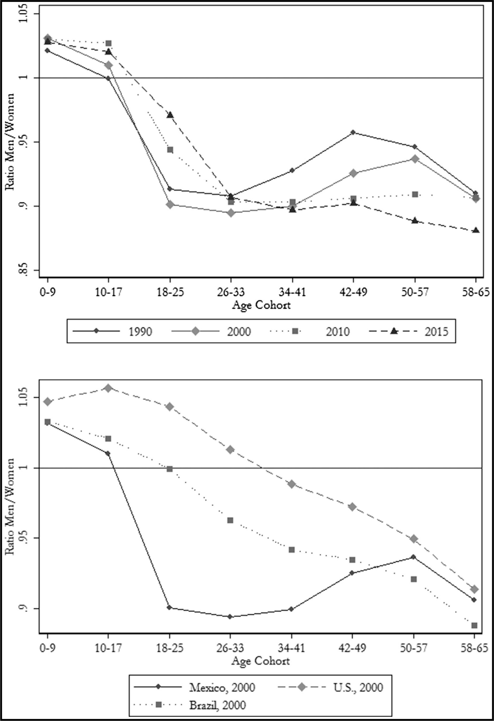
Figure 1
Sex ratios. Panel A: By census year and age group, Mexico. Panel B: Comparison of Mexico, United States, and Brazil.
Source: Brazil, Mexican, U.S. Census and ACS, accessed through IPUMS.
Table 1
Summary statistics
| N | Mean | Standard deviation | Minimum | Maximum | |
|---|---|---|---|---|---|
| Panel A: Explanatory variables of interest | |||||
| Sex ratio (men/women) | 640 | 0.93 | 0.05 | 0.81 | 1.13 |
| Predicted migration, EMIF | 640 | 0.21 | 0.17 | 0.01 | 0.95 |
| Predicted migration, ENE | 640 | 0.23 | 0.21 | 0.01 | 1.14 |
| Predicted migration, MC | 640 | 0.21 | 0.17 | 0.01 | 0.84 |
| Predicted migration, historical | 640 | 0.17 | 0.26 | 0.00 | 2.08 |
| Panel B: Labor market outcomes | |||||
| Women's labor force participation (%) | 640 | 0.35 | 0.12 | 0.05 | 0.62 |
| Women in white collar jobs (%) | 640 | 0.47 | 0.14 | 0.08 | 0.78 |
| Women in “brain” jobs (%) | 640 | 0.37 | 0.11 | 0.08 | 0.72 |
| Women in male-dominated professions (%) | 640 | 0.06 | 0.03 | 0.00 | 0.19 |
| Log (average earned monthly income), women | 640 | 7.99 | 0.26 | 7.27 | 8.91 |
| Women in top 25 of income (%) | 640 | 0.20 | 0.09 | 0.03 | 0.55 |
| Weekly hours worked, for women | 480 | 40.34 | 2.10 | 32.11 | 56.55 |
| Panel C: Other outcomes | |||||
| Women in blue collar jobs (%) | 640 | 0.53 | 0.14 | 0.22 | 0.92 |
| Women in “brawn” jobs (%) | 640 | 0.63 | 0.11 | 0.28 | 0.89 |
| Years of schooling, women | 640 | 8.00 | 2.43 | 1.57 | 12.98 |
| Lower secondary educated women (%) | 640 | 0.21 | 0.09 | 0.01 | 0.44 |
| Upper secondary educated women (%) | 640 | 0.11 | 0.07 | 0.002 | 0.29 |
| College-educated women (%) | 640 | 0.09 | 0.06 | 0.00 | 0.34 |
| Never married women (%) | 640 | 0.20 | 0.17 | 0.02 | 0.72 |
[i] Source: Hours worked are available only in the 1990, 2000, and 2010 census. Income is scaled to 2000 year peso values using CPI information provided by INEGI. See Section 2.2 for details on definition of labor market categories.
Table 2
First stage results
| (1) | (2) | (3) | (4) | (5) | (6) | (7) | |
|---|---|---|---|---|---|---|---|
| Actual | Random | Excluding | Excluding | Excluding | Excluding | Alternative | |
| Weights | Weights | Strong | Strong | Largest | Largest | Demand | |
| Connections | Connections2 | Receiving | Sending | CPS change | |||
| Predicted migration, EMIF | −0.228*** (0.028) | −0.034*** (0.011) | −0.295*** (0.030) | −0.228*** (0.028) | −0.460*** (0.063) | −0.301*** (0.037) | −0.211*** (0.038) |
| R2 | 0.61 | 0.57 | 0.62 | 0.61 | 0.59 | 0.61 | 0.55 |
| Predicted migration, ENE | −0.155*** (0.022) | −0.033*** (0.011) | −0.175*** (0.028) | −0.154*** (0.022) | −0.356*** (0.051) | −0.194*** (0.033) | −0.162*** (0.030) |
| R2 | 0.59 | 0.57 | 0.59 | 0.59 | 0.59 | 0.58 | 0.55 |
| Predicted migration, MC | −0.206*** (0.025) | −0.033*** (0.011) | −0.225*** (0.029) | −0.206*** (0.025) | −0.360*** (0.063) | −0.244*** (0.034) | −0.251*** (0.035) |
| R2 | 0.60 | 0.57 | 0.60 | 0.60 | 0.58 | 0.59 | 0.56 |
| Observations | 640 | 640 | 640 | 640 | 640 | 600 | 640 |
Notes: Dependent variable = Sex ratio (men/women). Robust standard errors, clustered at state–age group level in parentheses. All regressions include: state, year, age group fixed effects, percentage of the state's workforce employed in different industries by year (two-digit code). Column (3) excludes connections where both the U.S. and Mexican weights exceed 15%. Column (4) excludes connections where only the U.S. weight exceeds 50%. Column (5) excludes the largest receiving states: California, Texas, Arizona, and Florida. Column (6) excludes main sending states: Michoacán and Zacatecas (immigration rates greater than 10% of HHs).
Source: Mexican Census (MC), accessed through IPUMS.
Table 3
Second stage IV results
| (1) | (2) | (3) | (4) | (5) | (6) | (7) | |
|---|---|---|---|---|---|---|---|
| Female labor force participation | % Women in white collar jobs | % Women in “Brain” jobs | % Women in male-dominated professions | Log monthly earned income by women | % Women in top 25% income | Weekly hours worked by women | |
| Panel A: OLS | |||||||
| Sex ratio (men/women) | −0.419*** (0.064) | −0.232*** (0.053) | −0.457*** (0.046) | −0.042** (0.018) | −0.355*** (0.129) | −0.063 (0.040) | −1.241 (1.871) |
| R2 | 0.89 | 0.90 | 0.85 | 0.81 | 0.84 | 0.88 | 0.61 |
| Panel B: Weighting source EMIF | |||||||
| Sex ratio (men/women) | −0.693*** (0.145) | −0.676*** (0.152) | −1.065*** (0.141) | −0.020 (0.035) | −0.645** (0.292) | −0.125 (0.085) | 8.865* (5.039) |
| R2 | 0.89 | 0.88 | 0.81 | 0.81 | 0.84 | 0.88 | 0.58 |
| A-P F statistic | 66.12 | 66.12 | 66.12 | 66.12 | 66.12 | 66.12 | 41.60 |
| K-P chi squared | 52.40 | 52.40 | 52.40 | 52.40 | 52.40 | 52.40 | 41.47 |
| Panel C: Weighting source ENE | |||||||
| Sex ratio (men/women) | −0.666*** (0.167) | −0.815*** (0.192) | −1.167*** (0.176) | −0.048 (0.042) | −1.092** (0.465) | −0.396*** (0.152) | 11.499* (6.706) |
| R2 | 0.89 | 0.87 | 0.79 | 0.81 | 0.83 | 0.86 | 0.56 |
| A-P F statistic | 49.09 | 49.09 | 49.09 | 49.09 | 49.09 | 49.09 | 23.15 |
| K-P chi squared | 35.33 | 35.33 | 35.33 | 35.33 | 35.33 | 35.33 | 20.89 |
| Panel D: Weighting Source MC | |||||||
| Sex ratio (men/women) | −0.822*** (0.155) | −0.764*** (0.173) | −1.197*** (0.172) | −0.047 (0.039) | −0.871** (0.358) | −0.244** (0.103) | 13.474* (7.201) |
| R2 | 0.88 | 0.88 | 0.79 | 0.81 | 0.84 | 0.87 | 0.54 |
| A-P F statistic | 65.68 | 65.68 | 65.68 | 65.68 | 65.68 | 65.68 | 32.31 |
| K-P chi squared | 44.19 | 44.19 | 44.19 | 44.19 | 44.19 | 44.19 | 28.70 |
| Observations | 640 | 640 | 640 | 640 | 640 | 640 | 480 |
Notes: Robust standard errors, clustered at state–age group level in parentheses. All regressions include: state, year, age group fixed effects, percentage of the state's workforce employed in different industries by year (two-digit code). Hours worked are available only in the 1990, 2000, and 2010 census. See Section 2.2 for details on definition of categories. A-P stands for Angrist–Pischke F statistic. K-P stands for Kleinbergen–Paap rk LM chi-squared statistic.
Source: Mexican Census, accessed through IPUMS.
Table 4
Other outcomes, second stage, IV results
| (1) | (2) | (3) | (4) | (5) | (6) | (7) | |
|---|---|---|---|---|---|---|---|
| % Female in blue collar jobs | % Female in “Brawn” jobs | Years of schooling for women | % Women with lower secondary education (9) | % Women with upper secondary education (12) | % Women with college education (16+) | % Women who never married | |
| Panel A: OLS | |||||||
| Sex ratio (men/women) | 0.232*** (0.053) | 0.460*** (0.046) | −6.669*** (0.736) | −0.371*** (0.062) | 0.067** (0.028) | −0.136*** (0.028) | 0.033 (0.032) |
| R2 | 0.90 | 0.85 | 0.96 | 0.82 | 0.92 | 0.90 | 0.99 |
| Panel B: Weighting source EMIF | |||||||
| Sex ratio (men/women) | 0.676*** (0.152) | 1.077*** (0.141) | −12.733*** (1.614) | −0.708*** (0.140) | 0.381*** (0.070) | −0.034 (0.067) | −0.023 (0.065) |
| R2 | 0.88 | 0.81 | 0.95 | 0.80 | 0.89 | 0.89 | 0.99 |
| Panel C: Weighting source ENE | |||||||
| Sex ratio (men/women) | 0.815*** (0.192) | 1.168*** (0.176) | −17.306*** (2.528) | −1.108*** (0.193) | 0.281*** (0.074) | −0.109 (0.077) | 0.063 (0.085) |
| R2 | 0.87 | 0.79 | 0.93 | 0.73 | 0.90 | 0.90 | 0.99 |
| Panel D: Weighting source MC | |||||||
| Sex ratio (men/women) | 0.763*** (0.173) | 1.207*** (0.173) | −16.072*** (1.965) | −0.875*** (0.145) | 0.303*** (0.068) | −0.172*** (0.065) | 0.006 (0.073) |
| R2 | 0.88 | 0.79 | 0.94 | 0.78 | 0.90 | 0.90 | 0.99 |
| Observations | 640 | 640 | 640 | 640 | 640 | 640 | 640 |
Notes: Robust standard errors, clustered at state–age group level in parentheses. All regressions include: state, year, age group fixed effects, percentage of the state's workforce employed in different industries by year (two-digit code).
Source: Mexican Census, accessed through IPUMS.
Table 5
Second stage results: by education level
| (1) | (2) | (3) | (4) | (5) | (6) | (7) | |
|---|---|---|---|---|---|---|---|
| Female labor force participation | % Women in white collar jobs | % Women in “Brain” jobs | % Women in male-dominated professions | Log monthly earned income by women | % Women in top 25% income | Weekly hours worked by women | |
| Panel A: More than upper secondary (>12 years) | |||||||
| Sex ratio (men/women) | −1.857* (0.994) | −1.668 (1.113) | −2.039 (1.304) | −0.447 (0.333) | −2.373 (1.551) | −1.052 (0.694) | 32.611 (49.891) |
| R2 | −4.47 | −9.08 | −15.96 | −1.51 | −0.77 | −0.87 | −11.02 |
| A-P F statistic | 3.29 | 2.89 | 2.89 | 2.89 | 2.89 | 2.89 | 0.43 |
| Panel B: Upper secondary (10–12 years) | |||||||
| Sex ratio (men/women) | 0.006 (0.033) | 0.071* (0.042) | −0.059 (0.044) | 0.114*** (0.030) | 0.029 (0.094) | 0.077 (0.053) | −4.924*** (1.843) |
| R2 | 0.66 | 0.68 | 0.85 | 0.32 | 0.79 | 0.76 | 0.28 |
| A-P F statistic | 22.04 | 22.95 | 22.95 | 22.95 | 22.95 | 22.95 | 17.81 |
| Panel C: Lower secondary or less (9 or less) | |||||||
| Sex ratio (men/women) | −0.297*** (0.065) | −0.235*** (0.081) | −0.325*** (0.060) | 0.046*** (0.011) | 0.650*** (0.186) | 0.182*** (0.039) | 5.324* (2.912) |
| R2 | 0.86 | 0.84 | 0.89 | 0.76 | 0.86 | 0.82 | 0.69 |
| A-P F statistic | 56.16 | 56.16 | 56.16 | 56.16 | 56.16 | 56.16 | 29.44 |
Notes: Robust standard errors, clustered at state–age group level in parentheses. All regressions include the following controls: state, year, age group fixed effects, percentage of the state's workforce employed in different industries by year (two-digit code). Hours worked are available only in the 1990, 2000, and 2010 census. See Section 2.2 for details on definition of labor market categories. A-P stands for Angrist–Pischke F statistic. K-P stands for Kleinbergen–Paap rk LM chi-squared statistic.
Source: Mexican Census, accessed through IPUMS.
Table A1
Average Schooling by Job Type
| Year | 1990 | 2000 | 2010 | 2015 |
|---|---|---|---|---|
| Panel A: Years of education, mean | ||||
| White collar | 15.8 | 13.3 | 12.5 | 12.8 |
| Blue collar | 6.4 | 7.1 | 8.1 | 6.7 |
| Panel B: % with lower secondary education (9 years) | ||||
| White collar | 27.5 | 11.3 | 16.3 | 15.7 |
| Blue collar | 16.1 | 20.1 | 25.9 | 18.0 |
| Panel C: % with upper secondary education (12 years) | ||||
| White collar | 11.1 | 21.4 | 19.6 | 20.4 |
| Blue collar | 4.0 | 9.7 | 12.5 | 8.3 |
| Panel D: % with college education (16 or more years) | ||||
| White collar | 32.9 | 39.1 | 33.6 | 38.1 |
| Blue collar | 3.0 | 3.6 | 4.8 | 3.6 |
[i] Notes: Values are population weighted averages by census year. See Section 2.2 for details on definition of labor market categories.
Table A2
Sex Ratios and International Migration
| (1) | (2) | (3) | (4) | (5) | |
|---|---|---|---|---|---|
| Age Groups | 18–25 | 26–33 | 34–41 | 42–49 | 50–57 |
| International migration | |||||
| Panel A: 2000 | |||||
| % HH with international | −0.013*** (0.002) | −0.014*** (0.002) | −0.011*** (0.002) | −0.005* (0.003) | −0.006* (0.003) |
| R2 | 0.53 | 0.67 | 0.58 | 0.10 | 0.11 |
| Observations | 32 | 32 | 32 | 32 | 32 |
| Panel B: 2010 | |||||
| % HH with international | −0.029*** (0.005) | −0.032*** (0.006) | −0.019*** (0.005) | −0.016*** (0.005) | −0.021*** (0.007) |
| R2 | 0.56 | 0.49 | 0.34 | 0.26 | 0.25 |
| Observations | 32 | 32 | 32 | 32 | 32 |
| Homicides | |||||
| Panel C: 2010 | |||||
| Homicides per 10,000,000 | 0.043 (0.032) | 0.053 (0.039) | −0.001 (0.029) | 0.008 (0.028) | −0.003 (0.037) |
| R2 | 0.06 | 0.06 | 0.00 | 0.00 | 0.00 |
| Observations | 32 | 32 | 32 | 32 | 32 |
| Panel D: 2007–2010 | |||||
| Homicides per 10,000,000 | 0.012 (0.012) | 0.017 (0.015) | −0.005 (0.011) | 0.002 (0.011) | −0.004 (0.014) |
| R2 | 0.03 | 0.04 | 0.01 | 0.00 | 0.00 |
| Observations | 32 | 32 | 32 | 32 | 32 |
Notes: Standard errors in parenthesis.
Sources: Sex ratios and the percentage of households (HHs) with international migrants are from the Mexican Census, accessed through IPUMS. Homicides are from municipal death records compiled and made available by INEGI.
Table A3
Second stage results: robustness checks using EMIF weights
| (1) | (2) | (3) | (4) | (5) | (6) | (7) | |
|---|---|---|---|---|---|---|---|
| Female Labor Force Participation | % Women in White Collar Jobs | % Women in “Brain” Jobs | % Women in Male-Dominated Professions | Log Monthly Earned Income by Women | % Women in Top 25% Income | Weekly Hours Worked by Women | |
| Panel A: Historic weights | |||||||
| Sex ratio (men/women) | −0.128 (0.402) | −1.086 (0.667) | −1.111* (0.633) | −0.199 (0.166) | −6.912** (3.343) | −3.033** (1.491) | 3.215 (10.081) |
| A-P F statistic | 6.47 | 6.47 | 6.47 | 6.47 | 6.47 | 6.47 | 7.05 |
| Panel B: Movers included | |||||||
| Sex ratio (men/women) | −0.821*** (0.148) | −0.745*** (0.154) | −1.122*** (0.142) | −0.028 (0.035) | −0.589** (0.294) | −0.167* (0.087) | 9.058* (4.828) |
| A-P F statistic | 64.23 | 64.23 | 64.23 | 64.23 | 64.23 | 64.23 | 33.69 |
| Panel C: State-specific time trend | |||||||
| Sex ratio (men/women) | −0.714*** (0.125) | −0.669*** (0.097) | −1.070*** (0.098) | −0.019 (0.028) | −0.680*** (0.208) | −0.068 (0.067) | 7.997** (3.943) |
| A-P F statistic | 58.37 | 58.37 | 58.37 | 58.37 | 58.37 | 58.37 | 41.02 |
| Panel D: Age group and state time trends | |||||||
| Sex ratio (men/women) | 1.873*** (0.687) | −0.762** (0.321) | −0.504* (0.287) | −0.062 (0.087) | −0.495 (0.740) | 0.123 (0.286) | 27.850** (12.612) |
| A-P F statistic | 6.76 | 6.76 | 6.76 | 6.76 | 6.76 | 6.76 | 7.22 |
| Panel E: Additional state–year controls (FDI, Public Expenditure) | |||||||
| Sex ratio (men/women) | −0.756*** (0.123) | −0.671*** (0.097) | −1.069*** (0.098) | −0.033 (0.026) | −0.709*** (0.206) | −0.087 (0.065) | 6.996* (3.940) |
| A-P F statistic | 62.77 | 62.77 | 62.77 | 62.77 | 62.77 | 62.77 | 43.21 |
Table A4
Predicted Male Migration to the United States, year 2000
| Weighting Source | EMIF | ENE | MC | |
|---|---|---|---|---|
| (1) | (2) | (3) | ||
| 18–25 age group | Mean | 0.195 | 0.213 | 0.195 |
| Standard deviation | 0.136 | 0.177 | 0.137 | |
| 26–33 age group | Mean | 0.292 | 0.315 | 0.291 |
| Standard deviation | 0.215 | 0.269 | 0.214 | |
| 34–41 age group | Mean | 0.280 | 0.306 | 0.282 |
| Standard deviation | 0.200 | 0.259 | 0.198 | |
| 42–49 age group | Mean | 0.245 | 0.256 | 0.237 |
| Standard deviation | 0.160 | 0.210 | 0.157 | |
| 50–57 age group | Mean | 0.174 | 0.195 | 0.179 |
| Standard deviation | 0.113 | 0.163 | 0.113 | |
| Total | Mean | 0.235 | 0.257 | 0.237 |
| Standard deviation | 0.173 | 0.222 | 0.172 |
[i] Notes: First row number is the mean values across states. The second row number is the standard deviation.
[ii] Source: Authors’ calculations.