
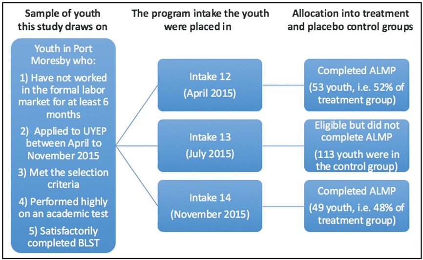
Figure 1
Process of selecting treatment and “placebo” control groups
Table 1
Questions that were asked to measure the main outcomes of interest
| Main outcome | Exact question |
|---|---|
| Formal sector employ- ment in last 6 months | Are you currently in or did you have a part-time or full-time wage job in the past 6 months in the formal sector? (i.e., regular or ongoing employment, not self-employment, or temporary work) |
| Average weekly wage from formal sector employment (Kina) | How much money do you earn/did you earn from this work each week? |
| Average number of hours worked in a week in for- mal sector employment | How many hours per week on average, do you work or did you work? |
| Earned cash in last 4 weeks | We know that you may earn cash from a range of different activities such as informal selling and temporary work. Now I want to consider everything that you have done in the last 4 weeks to earn cash, if you have earned cash. Did you earn any cash from any activities at all in the last 4 weeks? |
| Sought job in last 3 months | Have you sought any kind of paid job in the last 3 months? |
[i] Note: These questions were typically asked in the local dialect, Tok Pisin.
Table 2
Statistical balance across background characteristics
| (1) Control | (2) Treatment | t-test (2) - (1) | |||
|---|---|---|---|---|---|
| Variable | N | Mean/SE | N | Mean/SE | Difference |
| Age | 113 | 24.575 | 102 | 25.706 | 1.131* |
| [0.479] | [0.444] | ||||
| Share that are male | 113 | 0.558 | 102 | 0.647 | 0.09 |
| [0.047] | [0.048] | ||||
| Share that are married | 113 | 0.398 | 102 | 0.412 | 0.014 |
| [0.046] | [0.049] | ||||
| Total number of household members | 113 | 8.770 | 102 | 8.392 | –0.378 |
| [0.417] | [0.448] | ||||
| Female household members | 113 | 3.929 | 102 | 3.892 | –0.037 |
| [0.206] | [0.265] | ||||
| Male working household members | 113 | 1.044 | 102 | 1.029 | –0.015 |
| [0.102] | [0.115] | ||||
| Share with concrete floor | 113 | 0.053 | 102 | 0.078 | 0.025 |
| [0.021] | [0.027] | ||||
| Share with wood floor | 113 | 0.894 | 102 | 0.882 | –0.011 |
| [0.029] | [0.032] | ||||
| Years of education | 112# | 9.098 | 102 | 9.461 | 0.363 |
| [0.196] | [0.198] | ||||
[i] SE, standard errors in parentheses.
*p < 0.10, **p < 0.05, ***p < 0.01.
N refers to the number of observations.
#One people in the control group did not provide an answer to this question.
Table 3
Statistical balance across employment and job-seeking histories
| (1) Control | (2) Treatment | t-test (2) - (1) | |||
|---|---|---|---|---|---|
| Variable | N | Mean/SE | N | Mean/SE | Difference |
| Share that have never worked in formal | 113 | 0.743 | 102 | 0.794 | 0.051 |
| sector | [0.041] | ||||
| Number of formal sector jobs in lifetime | 113 | 0.389 | 102 | 0.343 | –0.046 |
| [0.058] | [0.065] | ||||
| Earn any money over last 6 months | 113 | 0.496 | 102 | 0.510 | 0.014 |
| [0.047] | [0.050] | ||||
| Sought a formal sector job in last | 113 | 0.150 | 102 | 0.147 | –0.003 |
| 3 months | [0.034] | ||||
| Sought any job last week | 113 | 0.080 | 102 | 0.069 | –0.011 |
| [0.026] | [0.025] | ||||
[i] SE, standard errors in parentheses.
*p < 0.10, **p < 0.05, ***p < 0.01.
Table 4
Statistical balance between placebo groups in intake 13 and intakes 12 and 14
| (1) Intake 13 Placebo group | (2) Intakes 12–14 Placebo group | Difference | |||
|---|---|---|---|---|---|
| Variable | N | Mean/SE | N | Mean/SE | (2) - (1) |
| Age | 134 | 23.522 | 224 | 23.415 | –0.107 |
| [0.449] | [0.323] | ||||
| Share that are male | 134 | 0.552 | 224 | 0.567 | 0.015 |
| [0.043] | [0.033] | ||||
| Share that are married | 134 | 0.425 | 224 | 0.366 | –0.059 |
| [0.043] | [0.032] | ||||
| Years of education | 120# | 7.442 | 198# | 6.949 | –0.492 |
| [0.256] | [0.202] | ||||
| Household members | 134 | 9.119 | 224 | 8.763 | –0.356 |
| [0.441] | [0.321] | ||||
| Female household members | 134 | 4.269 | 224 | 3.911 | –0.358 |
| [0.240] | [0.176] | ||||
| Male working household members | 134 | 1.239 | 224 | 1.196 | –0.042 |
| [0.129] | [0.088] | ||||
| Share with concrete floor | 134 | 0.060 | 224 | 0.062 | 0.003 |
| [0.021] | [0.016] | ||||
| Share with wood floor | 134 | 0.910 | 224 | 0.862 | –0.049 |
| [0.025] | [0.023] | ||||
[i] SE, standard errors in parentheses.
*p < 0.10, **p < 0.05, ***p < 0.01.
#Some respondents did not provide an answer to this question.
Table 5
Effect of the program on employment and job-seeking behavior
| (1) Control | (2) Treatment | t-test (2) - (1) | |||
|---|---|---|---|---|---|
| Variable | N | Mean/SE | N | Mean/SE | Difference |
| Formal sector employment in last 6 months | |||||
| Baseline | 113 | 0.000 | 102 | 0 | 0 |
| [0.000] | [0.000] | ||||
| Endline | 113 | 0.230 | 102 | 0.412 | 0.182*** |
| [0.040] | [0.049] | ||||
| Difference | 113 | 0.230 | 102 | 0.412 | 0.182*** |
| [0.040] | [0.049] | ||||
| Average weekly wage (Kina)# | |||||
| Baseline | 113 | 0.000 | 102 | 0 | 0 |
| [0.000] | [0.000] | ||||
| Endline | 113 | 87.673 | 102 | 123.255 | 35.582*** |
| [9.603] | [7.994] | ||||
| Difference | 113 | 87.673 | 102 | 123.255 | 35.582*** |
| [9.603] | [7.994] | ||||
| Average number of hours worked in a week# | |||||
| Baseline | 113 | 0.000 | 102 | 0 | 0 |
| [0.000] | [0.000] | ||||
| Endline | 113 | 23.805 | 102 | 36.843 | 13.038*** |
| [2.446] | [2.545] | ||||
| Difference | 113 | 23.805 | 102 | 36.843 | 13.038*** |
| [2.446] | [2.545] | ||||
| Earned cash in last 4 weeks | |||||
| Baseline | 113 | 0.381 | 102 | 0.343 | –0.037 |
| [0.046] | [0.047] | ||||
| Endline | 113 | 0.540 | 102 | 0.49 | –0.05 |
| [0.047] | [0.050] | ||||
| Difference | 113 | 0.159 | 102 | 0.147 | –0.012 |
| [0.062] | [0.064] | ||||
| Sought job in last 3 months | |||||
| Baseline | 113 | 0.150 | 102 | 0.147 | –0.003 |
| [0.034] | [0.035] | ||||
| Endline | 113 | 0.230 | 102 | 0.324 | 0.093 |
| [0.040] | [0.047] | ||||
| Difference | 113 | 0.080 | 102 | 0.176 | 0.097 |
| [0.051] | [0.060] | ||||
[i] SE, standard errors in parentheses.
*p < 0.10, **p < 0.05, ***p < 0.01.
#In formal sector employment.
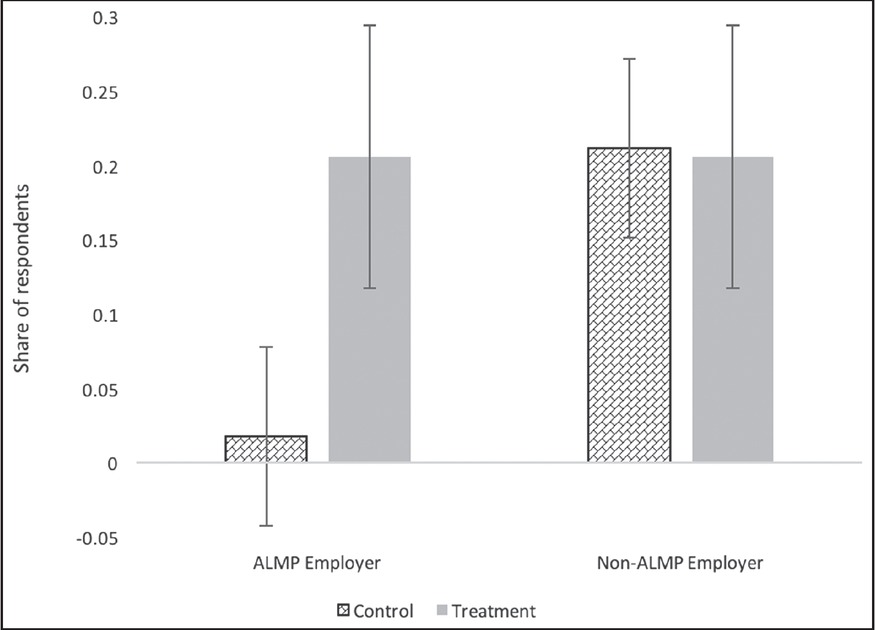
Figure 2
Impact of the program on formal employment by type of employer
Note: Two respondents in the control group claimed to be employed with their ALMP employer even though they did not complete the ALMP. This is why in the figure above the control group does not have 0% employment by ALMP employers.
Table 6
Results of the placebo test of the equal trends assumption
| (1) Intake 13 Placebo group | (2) Intakes 12–14 Placebo group | Difference | |||
|---|---|---|---|---|---|
| Variable | N | Mean/SE | N | Mean/SE | (2) - (1) |
| Formal sector employment in last 6 months | |||||
| Baseline | 134 | 0.000 | 224 | 0.000 | 0 |
| [0.000] | [0.000] | ||||
| Endline | 134 | 0.254 | 224 | 0.183 | –0.071 |
| [0.038] | [0.026] | ||||
| Difference | 134 | 0.254 | 224 | 0.183 | –0.071 |
| [0.038] | [0.026] | ||||
| Average weekly wage (Kina)# | |||||
| Baseline | 134 | 0.000 | 224 | 0.000 | 0 |
| [0.000] | [0.000] | ||||
| Endline | 134 | 70.090 | 224 | 60.045 | –10.045 |
| [8.114] | [6.185] | ||||
| Difference | 134 | 70.090 | 224 | 60.045 | –10.045 |
| [8.114] | [6.185] | ||||
| Average number of hours worked in a week# | |||||
| Baseline | 134 | 0.000 | 224 | 0.000 | 0 |
| [0.000] | [0.000] | ||||
| Endline | 134 | 18.754 | 224 | 15.348 | –3.406 |
| [2.196] | [1.528] | ||||
| Difference | 134 | 18.754 | 224 | 15.348 | –3.406 |
| [2.196] | [1.528] | ||||
| Earned cash in last 4 weeks | |||||
| Baseline | 134 | 0.321 | 224 | 0.339 | 0.018 |
| [0.040] | [0.032] | ||||
| Endline | 134 | 0.604 | 224 | 0.571 | –0.033 |
| [0.042] | [0.033] | ||||
| Difference | 134 | 0.284 | 224 | 0.232 | –0.051 |
| [0.053] | [0.044] | ||||
| Sought job in last 3 months | |||||
| Baseline | 134 | 0.052 | 224 | 0.094 | 0.042 |
| [0.019] | [0.020] | ||||
| Endline | 134 | 0.179 | 224 | 0.192 | 0.013 |
| [0.033] | [0.026] | ||||
| Difference | 134 | 0.127 | 224 | 0.098 | –0.029 |
| [0.036] | [0.032] | ||||
[i] SE, standard errors in parentheses.
*p < 0.10, **p < 0.05, ***p < 0.01.
#In formal sector employment.
Table A1
Difference in background characteristics between respondents who were re-interviewed and those that were not in the treatment group
| (1) Only in baseline survey | (2) In both baseline and Follow-up survey | t-test Difference | |||
|---|---|---|---|---|---|
| Variable | N | Mean/SE | N | Mean/SE | (2) - (1) |
| Age | 62 | 25.726 | 102 | 25.706 | 0.020 |
| [0.569] | [0.444] | ||||
| Share that are male | 62 | 0.661 | 102 | 0.647 | 0.014 |
| [0.061] | [0.048] | ||||
| Share that are married | 62 | 0.339 | 102 | 0.412 | –0.073 |
| [0.061] | [0.049] | ||||
| Years of education | 62 | 10.500 | 102 | 9.461 | 1.039*** |
| [0.172] | [0.198] | ||||
| Household members | 62 | 7.742 | 102 | 8.392 | –0.650 |
| [0.490] | [0.448] | ||||
| Female household members | 62 | 3.500 | 102 | 3.892 | –0.392 |
| [0.267] | [0.265] | ||||
| Male working household members | 62 | 0.871 | 102 | 1.029 | –0.158 |
| [0.125] | [0.115] | ||||
| Share with concrete floor | 62 | 0.065 | 102 | 0.078 | –0.014 |
| [0.031] | [0.027] | ||||
| Share with wood floor | 62 | 0.855 | 102 | 0.882 | –0.028 |
| [0.045] | [0.032] | ||||
[i] SE, standard errors in parentheses.
*p < 0.10, **p < 0.05, ***p < 0.01.
Table A2
Difference in background characteristics of respondents between who were re-interviewed and those that were not in the control group
| (1) Only in baseline survey | (2) In both baseline and follow-up survey | t-test Difference | |||
|---|---|---|---|---|---|
| Variable | N | Mean/SE | N | Mean/SE | (2) - (1) |
| Age | 78 | 24.051 | 113 | 24.575 | –0.524 |
| [0.467] | [0.479] | ||||
| Share that are male | 78 | 0.641 | 113 | 0.558 | 0.084 |
| [0.055] | [0.047] | ||||
| Share that are married | 78 | 0.321 | 113 | 0.398 | –0.078 |
| [0.053] | [0.046] | ||||
| Years of education | 77 | 9.584 | 112 | 9.098 | 0.486 |
| [0.243] | [0.196] | ||||
| Household members | 78 | 8.372 | 113 | 8.770 | –0.398 |
| [0.491] | [0.417] | ||||
| Female household members | 78 | 3.897 | 113 | 3.929 | –0.032 |
| [0.269] | [0.206] | ||||
| Male working household members | 78 | 1.231 | 113 | 1.044 | 0.187 |
| [0.138] | [0.102] | ||||
| Share with concrete floor | 78 | 0.128 | 113 | 0.053 | 0.075* |
| [0.038] | [0.021] | ||||
| Share with wood floor | 78 | 0.808 | 113 | 0.894 | –0.086* |
| [0.045] | [0.029] | ||||
[i] SE, standard errors in parentheses.
*p < 0.10, **p < 0.05, ***p < 0.01.
Table A3
Effect of the program using different econometric specifications
| OLS | OLS with controls | LOGIT | |
|---|---|---|---|
| Formal sector employment in last 6 months | 0.182*** | 0.164** | 0.851*** |
| –0.06 | –0.06 | –0.3 | |
| Average weekly wage (Kina)# | 35.582*** | 29.625** | N/A |
| –12.64 | –12.87 | N/A | |
| Average number of hours worked in a week# | 13.038*** | 12.359*** | N/A |
| –3.53 | –3.64 | N/A | |
| Earned cash in last 4 weeks | –0.012 | –0.014 | –0.077 |
| –0.09 | –0.09 | –0.27 | |
| Sought job in last 3 months | 0.097 | 0.129 | 0.447 |
| –0.08 | –0.08 | –0.29 |
[i] Standard errors in parentheses.
*p < 0.10, **p < 0.05, ***p < 0.01.
N/A: Not applicable because these outcomes are continuous.
#In formal sector employment.
Table A4
Differences in outcomes between youth in the control group and youth who were ineligible in intakes 12 and 14
| (1) Ineligible youth in intakes 12 and 14 | (2) Control group | t-test (2) - (1) | |||
|---|---|---|---|---|---|
| Variable | N | Mean/SE | N | Mean/SE | Difference |
| Formal sector employment in last 6 months | |||||
| Baseline | 224 | 0.000 | 113 | 0.000 | 0 |
| [0.000] | [0.000] | ||||
| Endline | 224 | 0.183 | 113 | 0.230 | 0.047 |
| [0.026] | [0.040] | ||||
| Difference | 224 | 0.183 | 113 | 0.230 | 0.047 |
| [0.026] | [0.040] | ||||
| Average weekly wage (Kina)# | |||||
| Baseline | 224 | 0.000 | 113 | 0.000 | 0 |
| [0.000] | [0.000] | ||||
| Endline | 224 | 60.045 | 113 | 87.673 | 27.628** |
| [6.185] | [9.603] | ||||
| Difference | 224 | 60.045 | 113 | 87.673 | 27.628** |
| [6.185] | [9.603] | ||||
| Average number of hours worked in a week# | |||||
| Baseline | 224 | 0.000 | 113 | 0.000 | 0 |
| [0.000] | [0.000] | ||||
| Endline | 224 | 15.348 | 113 | 23.805 | 8.457*** |
| [1.528] | [2.446] | ||||
| Difference | 224 | 15.348 | 113 | 23.805 | 8.457*** |
| [1.528] | [2.446] | ||||
| Earned cash in last 4 weeks | |||||
| Baseline | 224 | 0.339 | 113 | 0.381 | 0.041 |
| [0.032] | [0.046] | ||||
| Endline | 224 | 0.571 | 113 | 0.540 | –0.032 |
| [0.033] | [0.047] | ||||
| Difference | 224 | 0.232 | 113 | 0.159 | –0.073 |
| [0.044] | [0.062] | ||||
| Sought job in last 3 months | |||||
| Baseline | 224 | 0.094 | 113 | 0.150 | 0.057 |
| [0.020] | [0.034] | ||||
| Endline | 224 | 0.192 | 113 | 0.230 | 0.038 |
| [0.026] | [0.040] | ||||
| Difference | 224 | 0.098 | 113 | 0.080 | –0.019 |
| [0.032] | [0.051] | ||||
[i] SE, standard errors in parentheses.
*p < 0.10, **p < 0.05, ***p < 0.01.
#In formal sector employment.
Table A5
Differences in outcomes between youth in the control group and youth who were ineligible in intake 13
| (1) Ineligible youth in intake 13 | (2) Control group | t-test (2) - (1) | |||
|---|---|---|---|---|---|
| Variable | N | Mean/SE | N | Mean/SE | Difference |
| Formal sector employment in last 6 months | |||||
| Baseline | 134 | 0.000 | 113 | 0.000 | 0 |
| [0.000] | [0.000] | ||||
| Endline | 134 | 0.254 | 113 | 0.230 | –0.024 |
| [0.038] | [0.040] | ||||
| Difference | 134 | 0.254 | 113 | 0.230 | –0.024 |
| [0.038] | [0.040] | ||||
| Average weekly wage from (Kina)# | |||||
| Baseline | 134 | 0.000 | 113 | 0.000 | 0 |
| [0.000] | [0.000] | ||||
| Endline | 134 | 70.090 | 113 | 87.673 | 17.583 |
| [8.114] | [9.603] | ||||
| Difference | 134 | 70.090 | 113 | 87.673 | 17.583 |
| [8.114] | [9.603] | ||||
| Average number of hours worked in a week# | |||||
| Baseline | 134 | 0.000 | 113 | 0.000 | 0 |
| [0.000] | [0.000] | ||||
| Endline | 134 | 18.754 | 113 | 23.805 | 5.052 |
| [2.196] | [2.446] | ||||
| Difference | 134 | 18.754 | 113 | 23.805 | 5.052 |
| [2.196] | [2.446] | ||||
| Earned cash in last 4 weeks | |||||
| Baseline | 134 | 0.321 | 113 | 0.381 | 0.060 |
| [0.040] | [0.046] | ||||
| Endline | 134 | 0.604 | 113 | 0.540 | –0.065 |
| [0.042] | [0.047] | ||||
| Difference | 134 | 0.284 | 113 | 0.159 | –0.124 |
| [0.053] | [0.062] | ||||
| Sought job in last 3 months | |||||
| Baseline | 134 | 0.052 | 113 | 0.150 | 0.098*** |
| [0.019] | [0.034] | ||||
| Endline | 134 | 0.179 | 113 | 0.230 | 0.051 |
| [0.033] | [0.040] | ||||
| Difference | 134 | 0.127 | 113 | 0.080 | -0.047 |
| [0.036] | [0.051] | ||||
[i] SE, standard errors in parentheses.
*p < 0.10, **p < 0.05, ***p < 0.01.
#In formal sector employment.
Table A6
Differences in outcomes between youth in the treatment group and youth who were ineligible in intakes 12 and 14
| (1) Ineligible youth in intakes 12 and 14 | (2) Treatment group | t-test (2) - (1) | |||
|---|---|---|---|---|---|
| Variable | N | Mean/SE | N | Mean/SE | Difference |
| Formal sector employment in last 6 months | |||||
| Baseline | 224 | 0.000 | 102 | 0.000 | 0 |
| [0.000] | [0.000] | ||||
| Endline | 224 | 0.183 | 102 | 0.412 | 0.229*** |
| [0.026] | [0.049] | ||||
| Difference | 224 | 0.183 | 102 | 0.412 | 0.229*** |
| [0.026] | [0.049] | ||||
| Average weekly wage (Kina)# | |||||
| Baseline | 224 | 0.000 | 102 | 0.000 | 0 |
| [0.000] | [0.000] | ||||
| Endline | 224 | 60.045 | 102 | 123.255 | 63.210*** |
| [6.185] | [7.994] | ||||
| Difference | 224 | 60.045 | 102 | 123.255 | 63.210*** |
| [6.185] | [7.994] | ||||
| Average number of hours worked in a week# | |||||
| Baseline | 224 | 0.000 | 102 | 0.000 | 0 |
| [0.000] | [0.000] | ||||
| Endline | 224 | 15.348 | 102 | 36.843 | 21.495*** |
| [1.528] | [2.545] | ||||
| Difference | 224 | 15.348 | 102 | 36.843 | 21.495*** |
| [1.528] | [2.545] | ||||
| Earned cash in last 4 weeks | |||||
| Baseline | 224 | 0.339 | 102 | 0.343 | 0.004 |
| [0.032] | [0.047] | ||||
| Endline | 224 | 0.571 | 102 | 0.490 | –0.081 |
| [0.033] | [0.050] | ||||
| Difference | 224 | 0.232 | 102 | 0.147 | –0.085 |
| [0.044] | [0.064] | ||||
| Sought job in last 3 months | |||||
| Baseline | 224 | 0.094 | 102 | 0.147 | 0.053 |
| [0.020] | [0.035] | ||||
| Endline | 224 | 0.192 | 102 | 0.324 | 0.132*** |
| [0.026] | [0.047] | ||||
| Difference | 224 | 0.098 | 102 | 0.176 | 0.078 |
| [0.032] | [0.060] | ||||
[i] SE, standard errors in parentheses.
*p < 0.10, **p < 0.05, ***p < 0.01.
#In formal sector employment.
Table A7
Differences in outcomes between youth in the treatment group and youth who were ineligible in intake 13
| (1) Ineligible youth in intake 13 | (2) Treatment group | t-test (2) - (1) | |||
|---|---|---|---|---|---|
| Variable | N | Mean/SE | N | Mean/SE | Difference |
| Formal sector employment in last 6 months | |||||
| Baseline | 134 | 0.000 | 102 | 0.000 | 0 |
| [0.000] | [0.000] | ||||
| Endline | 134 | 0.254 | 102 | 0.412 | 0.158*** |
| [0.038] | [0.049] | ||||
| Difference | 134 | 0.254 | 102 | 0.412 | 0.158*** |
| [0.038] | [0.049] | ||||
| Average weekly wage (Kina)# | |||||
| Baseline | 134 | 0.000 | 102 | 0.000 | 0 |
| [0.000] | [0.000] | ||||
| Endline | 134 | 70.090 | 102 | 123.255 | 53.165*** |
| [8.114] | [7.994] | ||||
| Difference | 134 | 70.090 | 102 | 123.255 | 53.165*** |
| [8.114] | [7.994] | ||||
| Average number of hours worked in a week# | |||||
| Baseline | 134 | 0.000 | 102 | 0.000 | 0 |
| [0.000] | [0.000] | ||||
| Endline | 134 | 18.754 | 102 | 36.843 | 18.089*** |
| [2.196] | [2.545] | ||||
| Difference | 134 | 18.754 | 102 | 36.843 | 18.089*** |
| [2.196] | [2.545] | ||||
| Earned cash in last 4 weeks | |||||
| Baseline | 134 | 0.321 | 102 | 0.343 | 0.022 |
| [0.040] | [0.047] | ||||
| Endline | 134 | 0.604 | 102 | 0.490 | –0.114* |
| [0.042] | [0.050] | ||||
| Difference | 134 | 0.284 | 102 | 0.147 | –0.137* |
| [0.053] | [0.064] | ||||
| Sought job in last 3 months | |||||
| Baseline | 134 | 0.052 | 102 | 0.147 | 0.095** |
| [0.019] | [0.035] | ||||
| Endline | 134 | 0.179 | 102 | 0.324 | 0.144** |
| [0.033] | [0.047] | ||||
| Difference | 134 | 0.127 | 102 | 0.176 | 0.050 |
| [0.036] | [0.060] | ||||
[i] SE, standard errors in parentheses.
*p < 0.10, **p < 0.05, ***p < 0.01.
#In formal sector employment.