
I. Introduction
In recent days, emotion detection (ED) has gained significant interest in applications like adaptive virtual reality, mental health evaluation, intelligent robotics, and human-computer interaction. Emotions are the main factors of mental capabilities that describe the salience of events and objectives [1]. Positive emotions constitute method indications, while negative emotions (such as fear, disgust, etc.) constitute a warning of danger. Both play an important part in behavior, the decision-making process, thoughts, and communication with others [2]. The proper interpretation and detection of human emotions offer novel opportunities to design tailored user experiences and improve communication abilities [3]. Functional magnetic-resonance imaging (fMRI) is a noninvasive method to map neural activity through measuring blood-oxy-gen-level-dependent signals [4]. fMRI is broadly used for studying brain areas involved in affective conditions as well as emotion processing. Presenting good spatial resolution, the approach has been used in various research to identify and lateralize neural activity related to emotional processing and the underlying module in regulating and generating emotional replies [5]. Likewise, fMRI gives a more precise reflection of brain activity than variations in metabolic procedures may be tracked at the voxel level, compared with previous models such as electroencephalogram (EEG)-driven event-related synchronization as well as desynchronization [6]. The models have become indispensable in emotion system research by indicating the spatial and temporal limitations of affective processing. Therefore, a few of the models' drawbacks involve higher operational costs, restricted scalability, and low temporal resolution of magnetoencephalography (MEG) or EEG [7]. Despite this risk, fMRI has advanced research into detecting intricate neural pathways associated with emotional conditions.
Advances in these features are aided by research activities at the intersection of AI and cognitive neuroscience, where developments in neuroimaging models and deep learning (DL) methods have enhanced the quality of ED [8]. Affective neuroscience, which researches the biological and psychological modules underlying emotions, has been essential to shape ED models
Insights from cognitive science have increased the number of approaches analyzing the multidimensional features of emotions [9]. The main regions of study have been facial expression detection, which has a considerable contribution in psychiatry as well as digital psychology [10]. It offers objective measures of emotional conditions that can enable developments in human-computer interaction as well as mental health diagnostics [11]. Currently, the fast growth of AI, as well as cognitive neuroscience, has offered modern tools and methods. AI models, particularly DL models, have become essential for intricate pattern analytics, from image processing to series data modeling [12]. Neural networks (NNs) have become progressively common in neuroimage studies because of their robust performance in pattern classification and recognition challenges. Deep neural networks (DNNs) provide various benefits in neuroimage research, from analyzing macroscopic structural and fMRI information to microscopic connectivity patterns of NNs in animal research [13]. It is versatile across fields: image detection, larger-scale data analysis, and speech processing. In neuroscience, NNs allows comprehension of intricate brain functions by determining activation patterns through several cognitive as well as emotional conditions [14]. The convolutional neural network (CNN) structure is efficient in neuroimages since it can manage image distortions as well as recognize hierarchical feature extractions. They exceed individual performance in visual detection challenges to learn patterns correlated with various emotional as well as cognitive conditions [15]. This study develops an intelligent DL framework that analyzes brain activity from fMRI images, identifies important spatial patterns using capsule networks, captures temporal relationships using BiLSTM, and applies an attention mechanism to focus on the most relevant brain regions for accurate multi-class emotion classification.
It is important to note that the term “Optimal” in this study refers to the empirically optimized performance of the proposed model through systematic hyperparameter tuning using the Nadam optimizer. The optimality is not theoretically proven but is demonstrated through experimental comparisons, where the proposed model consistently outperforms several baseline and state-of-the-art approaches across multiple evaluation metrics.
a. Core contributions and section overview
To accurately detect and classify human emotional states from fMRI images, this article proposes the design and development of an Optimal Attention Deep Learning-based Multi-class Emotion Detection and Classification (OADL-MCEDC) framework. The proposed OADL-MCEDC methodology follows a comprehensive pipeline entailing fMRI preprocessing, feature map conversion, hybrid capsule feature representation, classification, and Nadam-based hyperparameter optimization. The performance assessment of the presented OADL-MCEDC technique is performed under a benchmark dataset, and the results are examined across different evaluation metrics. The core contributions of this manuscript are as follows:
Utilize a hybrid capsule network for feature extraction, which captures hierarchical, spatial, and functional patterns from fMRI feature maps, providing better representational capability.
Design an attention bidirectional long short-term memory (Attention-BiLSTM) classification, which models temporal relationships across brain regions while highlighting the most beneficial emotional cues, which enables precise multi-class emotion classification.
Integrate Nadam optimizer for hyperparameter tuning, which helps attain better convergence, enhanced classification model stability.
Evaluate the OADL-MCEDC model using bench-mark fMRI Emotion Recognition dataset. Comparative results specify that the proposed system performed better than other approaches across various performance metrics (accuracy, Precision, Recall, F-measure, and Matthews correlation coefficient [MCC]).
The manuscript is organized as follows: Section II offers a detailed review of the relevant literature, focusing on existing models, research gaps concerning ED and classification using fMRI images. Section III outlines the proposed system, including the pre-processing modules, the dimensionality reduction process, design of classification model, and the parameter optimization technique. In Section IV, the experimental results were outlined. This part encompasses an in-depth examination of the proposed system's performance on various measures. Finally, Section V concludes the papers by highlighting the key findings.
II. Prior Studies on fMRI-Based ED and Classification
This section outlines relevant studies focused on fMRI-based ED. [16] presented an effective dynamic AFER method that depends on a new spatial and temporal representation. The face landmarks are obtained, then every probable Euclidean distance is computed for modeling the spatial framework. For capturing temporal variations, 3 statistical metrics are used for every distance series. A feature selection phase that depends on the Extremely Randomized Trees (ExtRa-Trees) method is achieved for reducing the dimension and enhancing identification performance. The dynamic AFER method that uses imaging series could take the temporal evolution of facial expressions, then it frequently suffers from higher computational expenses, restraining its appropriateness for actual utilization. [17] examined thermal images as an alternative, utilizing the capability of capturing heat radiation as well as addressing lighting problems. An innovative method that integrates pre-trained techniques, especially EfficientNet variations, with Gray Wolf Optimizer (GWO) and several classification models for strong ED. The article provides the efficiency and consistency of the presented method for emotion classification in thermal imaging, creating a feasible method to solve the disadvantage of traditional visible-light-driven FER methods.
A new method is introduced for ED through a CNN DL method [18]. The model utilizes CNNs' hierarchical feature learning abilities to extract the discriminative features from the raw input information, allowing for precise emotion identification. Convolutional layers, accomplished by max-pooling operations, form a multi-layered CNN structure, particularly for spatial feature extraction, though they maintain the major hierarchical features. [19] presented a ViT-driven Dual-Polarity Memory Network (ViTDMN) that suggests a progressive emotion evocation procedure for improving the performance of IER. Particularly, early use of the ViT shallow features for polarity predictors simulates the polarity perspective throughout the progressive emotion evocation procedure. Therefore, building a DPMN to improving polarity emotion characteristics as discriminative signs for better guiding the fine-tuned classifiers. [20] suggested a Concept-guided Multi-level Attention Network (CMAN) that captures complete utilization of attribute feature idea for improving the image ED. To utilize many ideas to influence the removal of the emotional area, CMAN, as a multi-level structure, first calculates the semantic feature as directed by the feature from the whole step. Moreover, an adaptive fusion approach is presented to complement either semantic or attended visual features.
The authors in [21] established a new Unified Generative structure for Imaging Emotion Classification (UGRIE) that can concurrently model several emotion techniques and capture complex semantic relations among the emotion labels. This method uses an adaptable natural language template, changing the IEC challenge into a template-filling procedure that can be adapted easily to accommodate a wide variety of IEC tasks. To additionally improve the performance, devise a mapping module to effortlessly combine the multi-modal pre-trained technique CLIP with the text-generation pre-trained technique BART. [22] presented a region-driven multi-scale system, learning attributes for the local effective area and a wide context for affective image detection. This method consists of an effective area recognition mechanism as well as a multi-scale feature learning mechanism. The class activation mapping approach is utilized for generating pseudo affective areas from a pre-trained DNN to train the recognition mechanism. For the affective area output by the recognition mechanism, three-scale feature extraction is performed and then encoded by a kernel-driven graph attention system to classify the last emotion. [23] examined the efficiency of CNNs in identifying imagery into pre-defined classes, emphasizing developments in automatic image detection models. This method is intended to develop a strong CNN technique that could precisely classify and identify imagery that depends on the content, which has important suggestions for domains that require automatic image examination. To demonstrate the ability to handle intricate pattern detection challenges, the ability of CNNs in transforming image processing applications is examined. [24] proposed a machine vision-based system for automatic detection of missing rail fasteners using a support vector machine (SVM) classifier with Gabor transform and texture-based feature extraction such as GLCM, LBP, and DWT. The study highlights the effectiveness of traditional machine learning approaches in image classification tasks involving preprocessing, feature extraction, and supervised learning.
Table 1 offers a comparison analysis of existing approaches based on their research gap, methodologies, and outcomes.
Table 1:
Summary of multiclass emotion recognition techniques
| References | Years | Research gaps | Methodologies | Outcomes |
|---|---|---|---|---|
| [16] | 2025 | Current methods lack simple, fast use of spatial-temporal features for real-time ED. | SVM, KNN approaches. | Recognition rates of 94.65%, 93.98%, and 75.59%. |
| [17] | 2025 | FER methods lack thermal-based deep models for reliable, lighting-independent, accurate emotion recognition. | EfficientNet, GWO, SVM, KNN, RF, and Gradient Boosting techniques. | Accuracy of 91.42% and 99.48%. |
| [18] | 2025 | CNN-based emotion recognition struggles with imbalanced data and unreliable real-time performance across environments today. | CNN models. | Accuracy of 97%. |
| [19] | 2025 | Existing IER methods ignore progressive emotion perception and lack mechanisms to model emotions. | ViT and DPMN. | Accuracy of 75.35% and 66.84%. |
| [20] | 2024 | Existing methods lack concept-guided attention to accurately identify truly emotion-relevant regions in images. | CMANet model. | Gains an improved solution. |
| [21] | 2023 | Existing IEC methods cannot unify different emotion models or handle complex semantic relationships effectively. | Unified generative framework. | Achieves a better outcome. |
| [22] | 2022 | Existing methods overlook broad contextual features around affective regions, limiting robust emotion representation learning. | GCN, GAT, and RPN models. | Recognition rate of 87.47%, 76.05%, and 76.50%. |
| [23] | 2024 | CNN models still suffer from limited accuracy and lack deeper feature extraction for complex image classification tasks. | CNN techniques. | Accuracy of 62.2%. |
Recent studies have further contributed to DL-based classification and feature fusion methods. [25] proposed a Vision Transformer-embedded feature fusion model combined with pre-trained transformers for keratoconus disease classification, demonstrating improved feature representation capability using transformer-based architectures. This highlights the effectiveness of attention-based transformer models in medical image analysis tasks.
Similarly, [26] developed a deep CNN-based framework for malware detection and mitigation, showcasing the strength of CNN architectures in learning discriminative patterns from complex data-sets. Their approach emphasizes the robustness of DL models in classification problems across different domains.
In addition, [27] investigated genetic associations between common lung diseases and lung cancer progression using bioinformatics and machine learning techniques, demonstrating how ML-based feature extraction and predictive modeling can support disease analysis and early prediction in biomedical applications.
III. Proposed Workflow
This study presents an effective and attention-based DL architecture for multi-class ED and classification using fMRI imagery. Figure 1 presents the high-level workflow of the OADL-MCEDC system. As shown in Figure 1, the proposed model encompasses three major stages: image preprocessing, hybrid capsule-based feature representation, and emotion state classification using Attention-BiLSTM. Each stage is carefully designed to ensure accurate emotion state classification using fMRI images.
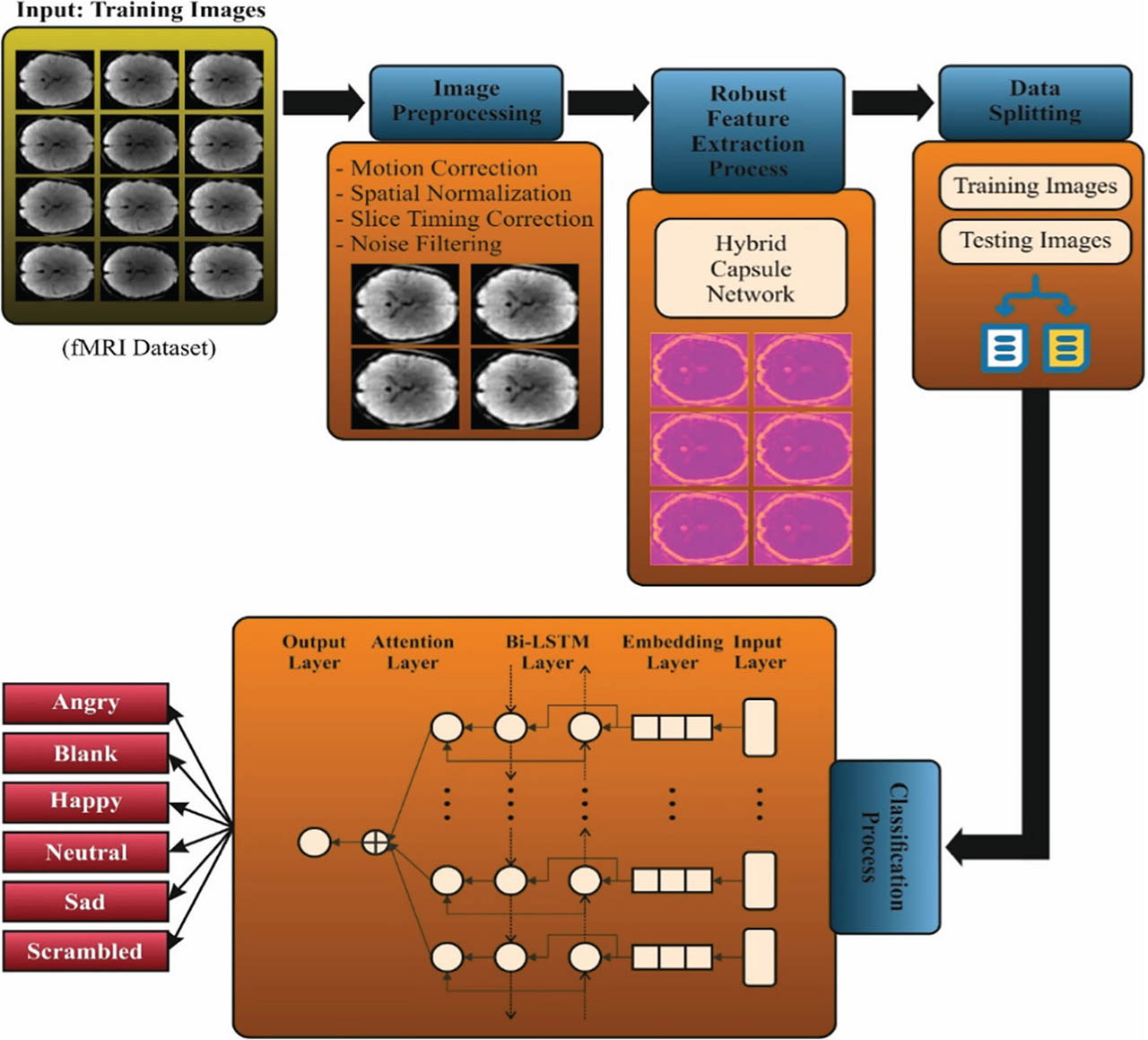
Figure 1:
High-level workflow of the proposed OADL-MCEDC approach. fMRI, functional magnetic-resonance image; OADL-MCEDC, Optimal Attention Deep Learning-based Multi-class Emotion Detection and Classification.
a. Image preprocessing
At the initial stage, preprocessing techniques were performed to improve the quality and consistency of the input fMRI data. The following operations were applied:
Motion Correction: A rigid body transformation was used to compensate for subject movement between successive volumes. Head motion was quantified using framewise displacement (FD) in both translation and rotation, and samples exceeding a threshold of 1.5 mm or 1.5° were excluded.
Slice Timing Correction: This step addresses differences in acquisition time across fMRI slices. An interpolation-based approach was applied to align voxel signals to a common temporal reference within the same repetition time (TR).
Spatial Normalization: Individual brain scans were transformed into a standard anatomical space using the Montreal Neurological Institute (MNI) atlas through nonlinear transformation, ensuring inter-subject consistency.
Spatial Smoothing and Noise Filtering: A Gaussian kernel with full width at half maximum (FWHM) was applied to enhance the signal-to-noise ratio (SNR) and reduce high-frequency noise. Additionally, temporal high-pass filtering was used to remove low-frequency drift and physiological noise caused by respiration and scanner instability.
These preprocessing steps ensure that the fMRI data are standardized, noise-reduced, and suitable for reliable feature extraction and subsequent emotion classification. The preprocessing steps include motion correction, where rigid body transformation compensates for subject movement between volumes, excluding samples with FD exceeding 1.5 mm or 1.5°. Slice timing correction aligns voxel signals to a common temporal reference using interpolation to address timing differences across fMRI slices. Noise filtering is performed using a Gaussian kernel for spatial smoothing and temporal high-pass filtering to remove low-frequency drift and physiological noise. Each of these preprocessing steps is critical to ensure that the fMRI data are standardized, noise-reduced, and suitable for reliable feature extraction and subsequent emotion classification.
b. Feature extraction
After preprocessing, the preprocessed fMRI images are converted into feature maps and fed into the hybrid capsule network for deep feature representation. This capsule-based network extracts localized as well as hierarchical activation patterns in the brain. This allows the extraction of discriminative and effective representations important for classifying various emotional states.
c. Emotion classification
In the final stage, the extracted capsule features are passed into an Attention-BiLSTM network for emotion classification. The BiLSTM component learns temporal and bidirectional relations across sequential fMRI activations. At the same time, the integrated attention mechanism assigns greater importance to brain regions that contribute most strongly to emotional expression. This integration enables the system to deliver accurate and robust multi-class emotion classification.
d. Image preprocessing
The proposed system preprocessed the input images with motion correction, spatial normalization, slice timing correction, and noise filtering techniques to ensure high-quality fMRI inputs. These preprocessed fMRI images are converted into feature maps for analysis.
d.i. Motion correction
It intends to verify the head signal distribution and eliminate participants with extreme head motions from supplementary studies [28]. Compute FD in rotation and translation based upon rigid body alteration. The formulation for FD at tth time is mentioned below:
Here, x, y, and z denote the 3 translation directions, hp signifies the head position parameters, and α, β, and γ signify the 3 rotation directions. Design the distribution of the greatest FD across every participant. A pre-specified threshold of largest FD >1.5 mm or 1.5° is applied for eliminating the participants. However, the threshold depends upon the feature sample.
d.ii. Spatial normalization
Spatial normalization is utilized for aligning the brain's shape, size, and location across participants for turning the brain imageries into a standardized template space. The functional images are standardized over combined segmentation of images, which is tracked by a normal brain template called MNI. Next, a Gaussian kernel is applied alongside a FWHM for enhancing the spatial smoothing. To split the brain into ROIs, an automatic functional labeling has been selected as the normal brain atlas. As dissimilar cognitive conditions arise, the ROIs function together when the system varies. Normalization employs a nonlinear transformation W, which maps an individual brain coordinate x to template coordinates xt.
d.iii. Slice timing correction
Almost all fMRI data are gathered through 2D MRI acquisition, where the information is attained with the timing and equally spread over the repetition time (TR). In a few situations, the slices are attained in order of descending or ascending. In another recognized technique, interleaved acquisition is attained successively. These alterations are difficult for the study of fMRI data. The main objective of slice timing correction is to alter the voxel time-series so that usual reference timing occurs for every voxel. Slice timing correction compensates for time differences among slice acquisitions. For every voxel signal S (t), the corrected signal is calculated below:
Here, Δts denotes a temporal offset for slice s.
d.iv. Noise filtering
fMRI signals cover physical noise (heartbeat, respiration), thermal noise, and scanner drift. The removal of noise is naturally executed utilizing:
Time-based high-pass filtering:
whereas h(t) denotes a lower-frequency kernel, eliminating slow drifts.d.v. Spatial smoothing
A Gaussian kernel Gσ is employed for enhancing SNR:
e. Hybrid capsule network-driven feature representation
To achieve reliable feature extraction, a hybrid capsule network is utilized to extract discriminative patterns crucial for ED.
e.i. CNN approach
The CNN's purpose is to study how the output and input data are mapped. As the databases are volumetric, using two-dimensional-CNN and three-dimensional CNN makes it probable for attaining the maximum precision [29]. For two-dimensional CNN, a sequence of matrix multiplication called a kernel filter with a dimension of sample (Pi, Qj) in layer i was tracked by a summation process. To enlarge, , an output placed at (a, b) for feature mapping j and layer i is formulated below:
Here, tanh denotes a nonlinearity process applied to the biases (bij) and kernel output. m and represents a kernel output positioned at (x, y) for feature mapping k and an index parameter in (i − 1)th layer, respectively. Generally, a convolution layer output is a feature mapping, signifying numerous attributes studied from an input image. The block of convolution was achieved by a sub-sampling or pooling process. In the pooling process, sections were formed for every value of pixel, but only the highest pixel value was retained. Lastly, the higher-level is performed utilizing fully connected (FC) layer, convolution, and max pooling layers. In a FC layer, neurons were linked to each activation.
Likewise, since that Ri denotes a 3rd dimension of kernels in 3D-CNN, an output positioned at (a, b, c) for feature mapping j and the layer i is expressed in Eq. (8), while denotes a kernel output at ( x, y, z).
e.ii. CapsNet approach
In terms of neuron structure, whole structure, propagation, and inter-layer distribution models, there is a major dissimilarity between CapsNet and conventional CNN methods. The capsule neuron is a crucial component in CapsNet. The parameters are employed as inputs and outputs with the conventional neuron structure. Capsule networks are intended for attaining an opposite illustration. Capsules obtain an image and recognize as well as its instantiation parameter. So, they are described as functions, which are efficient for forecasting the instantiation parameter for any chosen article at an exact position. The assessed probability was signified through the activation vector length. Similarly, the activation vector discloses an object instantiation parameter. For executing a prediction, the dot product was applied. The hierarchy was attained effortlessly by observing as an activation path and understanding the portions that fit together with higher accuracy.
The structure of CapsNet is straightforward. It comprises numerous layers, i.e., primary capsule, convolution layers, DigitCaps, and FC layers. A digit image was served, and every layer includes a convolution (Conv1 and Conv2 with dissimilar strides and similar kernels). ReLU was employed for activating the typical convolutional layers. As a result, Convl and Conv2 yield dissimilar feature mappings. The main layer is molded by redesigning the feature map and answerable for building the structure of corresponding vector.
Likewise, the DigitCaps layer signifies an output layer for capsules. For the encoding part, the loss function is defined, while the FC layers were used to rebuild the imageries (decoding part) to perform as a network regularization that averts overfitting. The DR model was used among the DigitCaps and primary capsules for upgrading the computations and parameters essential among the full connection. Moreover, the DR is applied alongside the conventional back-propagating model.
e.iii. Dynamic routing algorithm
As per Eq. (9), the main capsule ui (i = 1,…,1,152) was multiplied by a weighted matrix Wij for forecasting the capsule output in ten DigitCaps (j = 1,…,10). The output of 16D capsules was defined by increasing the multiplication of 8D primary capsules ui and weighted matrix Wij. So, Wij dimension will be [16 × 8].
In the training phase, one group of an input image at every iteration was served to a layer of input. Subsequently, the dual convolutional layers and reforming was achieved. Next, at primary iteration (r = 1), the log likelihood bij is fixed to 0 for every predicted output . Afterward, the softmax function was executed for every main capsule:
Subsequently, a weighted sum of forecasts was calculated in Eq. (12), besides employing the squashing function in Eq. (13). The squashing function compresses and nonlinearized the vector, executes the neuron's capsule. Here, an activation function comprises dual-parts, such as the unit length, which is answerable for defending the vector length among 0 and 1, and an additional scaling is answerable for protecting the vector path:
The design choices of the capsule network, alternative activation functions such as ReLU, sigmoid, and tanh were initially considered; however, they were found unsuitable for capsule representations as they either fail to preserve vector magnitude information or introduce saturation effects that reduce feature discriminability. The squashing function was therefore selected as it nonlinearly scales vectors, compressing short vectors toward zero while limiting long vectors to a value close to one, thereby enabling vector length to represent feature presence probability while preserving directional information, which is essential for capturing subtle fMRI-based emotion variations. In addition, dynamic routing was adopted instead of simpler routing mechanisms due to its iterative agreement process between lower- and higher-level capsules, which enhances hierarchical feature learning and improves modeling of complex spatial dependencies in brain activation data, leading to more stable convergence and improved classification performance.
Subsequently, by employing the dot product in Eq. (14), the prediction among upper and lower capsules was executed. Afterward, the routing weight established in Eq. (15) is upgraded:
Hence, in the topmost layer, an image model is intended with a single capsule per class. Next, it is essential to add a measuring layer for computing the length of the highest-layer activation vector. However, Hinton applied a margin loss Lk in Eq. (16) for permitting manifold classes in an image. As per this calculation, if class k is perceived, then an output for consistent capsule length must be higher than or equivalent to 0.9.
To let manifold class labels, the margin loss Tk = 1 was diminished if and only if kth class was present.
Once the routing weight bi,j, Updated is upgraded, the backpropagation will begin. In an original CapsNet, they are united as a decoding network at the top of the CapsNet. The overall loss in Eq. (17) denotes an outline of reconstruction and margin losses. To certify that the controlling loss is the margin loss, the reconstruction loss was measured with a smaller coefficient.
e.iv. Hybrid CapsNet
In an original CapsNet, the method was intended for traditional images of computer vision. Hence, to attain an appropriate classification method, the important system of the developed HCapsNet was separated into three sections, which are given below:
Dimension Reduction: Initially, principal component analysis (PCA) was employed on labeled database for reducing the spectrum redundancy. It condenses and decreases several spectral bands. Next, the corresponding image was separated into patches around central pixel without feature engineering. Lastly, 2D and 3D CNNs were employed for extracting the spectral-spatial feature mapping.
Capsule Network: Here, an output was initially redesigned into nD vector ui (i = 1, …, I). Then, it was increased by weighted matrix Wij to forecast the capsules for ClassCapsule . whereas J and I denote the number of main capsules and class labels, respectively, and m indicates the length of vector. Next, the weighted sum Sj is computed, tracked by the squash function. Afterward, the DR procedure is achieved for directing the most associated capsule in PrimaryCaps to Class-Capsule. Lastly, a model is intended in the topmost layer with a single capsule.
Decoder: Here, an extra reconstruction loss was employed for driving the subsequent level capsule named ClassCapsule for encrypting the instantiation parameter from input data. Even though the decoding works equally to a regularized one, inserting the margin loss is a must to avert overfitting throughout the training. Figure 2 signifies the architecture of the hybrid capsule network.
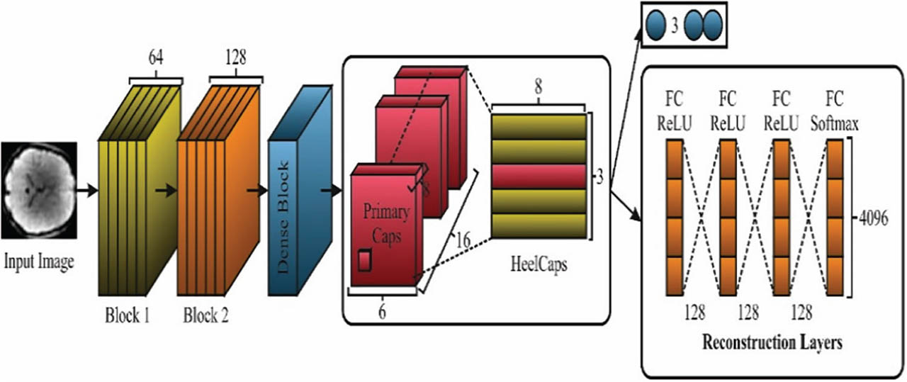
Figure 2:
Architecture of hybrid capsule network. FC, fully connected.
f. Emotion state classification module
An Attention-BiLSTM network is designed to classify emotional states effectively. The LSTM network belongs to the family of RNNs, which was mainly intended to address the issue of gradient vanishing when the methods are trained for learning longer-distance successive data [30]. To tackle this issue, gating mechanisms such as input, forget, and output gates as well as memory cell are applied for controlling data flow. LSTM is capable of upholding and updating its cell state over a longer time of period. The design of LSTM enables it to efficiently handle numerous processes from language processing to predicting time series. The formulation of forget gate was expressed below:
Here, δ represents the activation function of sigmoid, Xi means an input vector at time-step, t and ht−1 signifies a hidden vector from the preceding time-step t−1. Wf and bf are set randomly and slowly upgraded when the method trains. The arithmetical representation of input as well as output gates is stated below:
The candidate memory cell (Lt) donates to alter data in present cell states (Ct). The present cell state (Ct) and output Ot are employed for creating the existing hidden layer (HL) (ht), as below:
The attention layer accepts HL H = [h1, h2, h3,…, hn] reimbursed from the LSTM layer. Then, the HLs vectors hk are nonlinearly converted to form an activated output U = [u1, u2, u3,…, un] utilizing the Tanh function:
Here, Wk signifies weight matrix and bk denotes the offset mass at time-step k. Specific operational features throughout the shield tunneling procedure have an important influence on the location and direction. The attention module is employed for creating an attention weight matrix αk = [α1,α2,α3,α4 …,αn].
where αk denotes the normalized attention weight at time-step k and us represents a time series attention matrix. Lastly, for every input sample, a calculated weighted number of HLs is attained to form an attention vector V.The hyperparameters of the proposed OADL-MCEDC framework were configured as follows:
f.i. Epoch optimization
The number of training epochs was systematically optimized by evaluating model performance at 500, 1,000, 1,500, 2,000, 2,500, and 3,000 epochs. As demonstrated in Table 2, 3,000 epochs achieved the highest accuracy (98.33%) and was therefore selected for the final model.
Table 2:
Classifier recognition of OADL-MCEDC method on various epochs
| Class labels | Accury | Precin | Recall | Fmeasure | MCC |
|---|---|---|---|---|---|
| Epoch – 500 for multi-classes (angry, blank, happy, neutral, sad, scrambled) | 94.73 | 81.40 | 88.67 | 84.88 | 81.80 |
| 95.40 | 85.77 | 86.80 | 86.28 | 83.52 | |
| 93.58 | 76.96 | 87.73 | 81.99 | 78.35 | |
| 96.80 | 90.95 | 89.73 | 90.34 | 88.42 | |
| 90.71 | 74.85 | 66.67 | 70.52 | 65.18 | |
| 94.02 | 86.38 | 76.13 | 80.94 | 77.62 | |
| Average | |||||
| 94.21 | 82.72 | 82.62 | 82.49 | 79.15 | |
| Epoch – 1,000 for multi-classes (angry, blank, happy, neutral, sad, scrambled) | 95.82 | 84.69 | 91.47 | 87.95 | 85.52 |
| 97.09 | 90.89 | 91.73 | 91.31 | 89.56 | |
| 95.80 | 84.59 | 91.47 | 87.89 | 85.45 | |
| 97.33 | 92.68 | 91.20 | 91.94 | 90.34 | |
| 93.04 | 81.08 | 76.00 | 78.46 | 74.37 | |
| 95.76 | 91.04 | 82.67 | 86.65 | 84.27 | |
| Average | |||||
| 95.81 | 87.49 | 87.42 | 87.37 | 84.92 | |
| Epoch – 1,500 for multi-classes (angry, blank, happy, neutral, sad, scrambled) | 96.44 | 86.78 | 92.80 | 89.69 | 87.62 |
| 97.38 | 91.69 | 92.67 | 92.18 | 90.60 | |
| 97.29 | 89.55 | 94.80 | 92.10 | 90.52 | |
| 97.84 | 94.42 | 92.53 | 93.47 | 92.18 | |
| 95.11 | 87.32 | 82.67 | 84.93 | 82.06 | |
| 96.64 | 92.72 | 86.67 | 89.59 | 87.67 | |
| Average | |||||
| 96.79 | 90.41 | 90.36 | 90.33 | 88.44 | |
| Epoch – 2,000 for multi-classes (angry, blank, happy, neutral, sad, scrambled) | 96.67 | 88.07 | 92.53 | 90.25 | 88.28 |
| 97.56 | 92.33 | 93.07 | 92.70 | 91.23 | |
| 97.80 | 91.68 | 95.47 | 93.53 | 92.24 | |
| 97.87 | 94.07 | 93.07 | 93.57 | 92.29 | |
| 95.49 | 87.21 | 85.47 | 86.33 | 83.64 | |
| 97.11 | 94.41 | 87.87 | 91.02 | 89.39 | |
| Average | |||||
| 97.08 | 91.30 | 91.24 | 91.23 | 89.51 | |
| Epoch – 2,500 for multi-classes (angry, blank, happy, neutral, sad, scrambled) | 97.51 | 91.00 | 94.40 | 92.67 | 91.19 |
| 98.38 | 94.60 | 95.73 | 95.16 | 94.19 | |
| 98.51 | 93.06 | 98.40 | 95.66 | 94.81 | |
| 98.49 | 96.58 | 94.27 | 95.41 | 94.52 | |
| 97.29 | 93.85 | 89.60 | 91.68 | 90.09 | |
| 98.00 | 95.71 | 92.13 | 93.89 | 92.71 | |
| Average | |||||
| 98.03 | 94.14 | 94.09 | 94.08 | 92.92 | |
| Epoch – 3,000 for multi-classes (angry, blank, happy, neutral, sad, scrambled) | 97.93 | 93.05 | 94.67 | 93.85 | 92.62 |
| 98.62 | 95.62 | 96.13 | 95.88 | 95.05 | |
| 98.62 | 93.99 | 98.00 | 95.95 | 95.15 | |
| 98.73 | 97.14 | 95.20 | 96.16 | 95.41 | |
| 97.84 | 94.54 | 92.40 | 93.46 | 92.18 | |
| 98.24 | 95.77 | 93.60 | 94.67 | 93.63 | |
| Average | |||||
| 98.33 | 95.02 | 95.00 | 95.00 | 94.01 |
f.ii. Hyperparameter configuration
All hyperparameters were set based on standard configurations from capsule network literature [29, 30] for neuroimaging classification tasks. The complete configuration is as follows:
Optimizer: Nadam
Learning rate: 0.002 (Nadam default)
Batch size:** 32
Capsule dimension:** 16D (as specified in Eq. 10)
Dynamic routing iterations: 3
Capsule network filters: 128
BiLSTM hidden units: 128
Dropout rate: 0.5
Nadam is an optimizer method, which is robust stochastic optimizer needs only a primary order gradient with small memory necessity. It is simple to execute, effectual in computation, and requires less memory desires [31]. However, it does not vary for diagonal gradient measures and is well suitable for huge issues with parameters or data. Nadam employed preserved Adam's momentum component that is an advantage. It formed a substitution that amplified the speed of convergence and the model's excellence. Nadam is fragment of stochastic gradient descent. It works well in DL for updating the bias and weight values to reduce the result-ant loss. In the back-propagation procedure, the Nadam algorithm was employed for updating the weights and bias on wt+1 parameter, where t represents a time-step and wt denotes a current weight. L indicates a value of loss function, while the parameter values of decay β and rate of learning a are adaptable. Furthermore, an average exponential gesture of gradient V and squared gradient S began with 0.
IV. Results and Evaluation
In this section, the data used along with the metrics and the result analysis of the proposed model is presented.
a. Dataset overview
The performance validation (VALD) of the proposed model is studied under the fMRI dataset for Emotion Recognition dataset [32]. The dataset includes 4,500 sample images under 6 categories as shown in Table 3. Figure 3 illustrates the sample images. Figure 4 exhibits the preprocessed images, extracted feature maps, and GradCAM visualizations.
Table 3:
Details of dataset
| Emotions | Sample images |
|---|---|
| Angry | 750 |
| Blank | 750 |
| Happy | 750 |
| Neutral | 750 |
| Sad | 750 |
| Scrambled | 750 |
| Total Images | 4,500 |
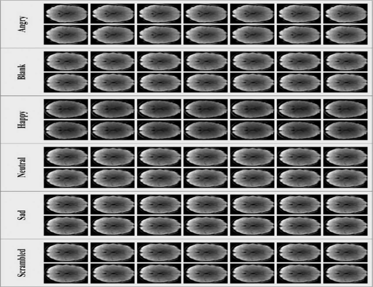
Figure 3:
Sample images.
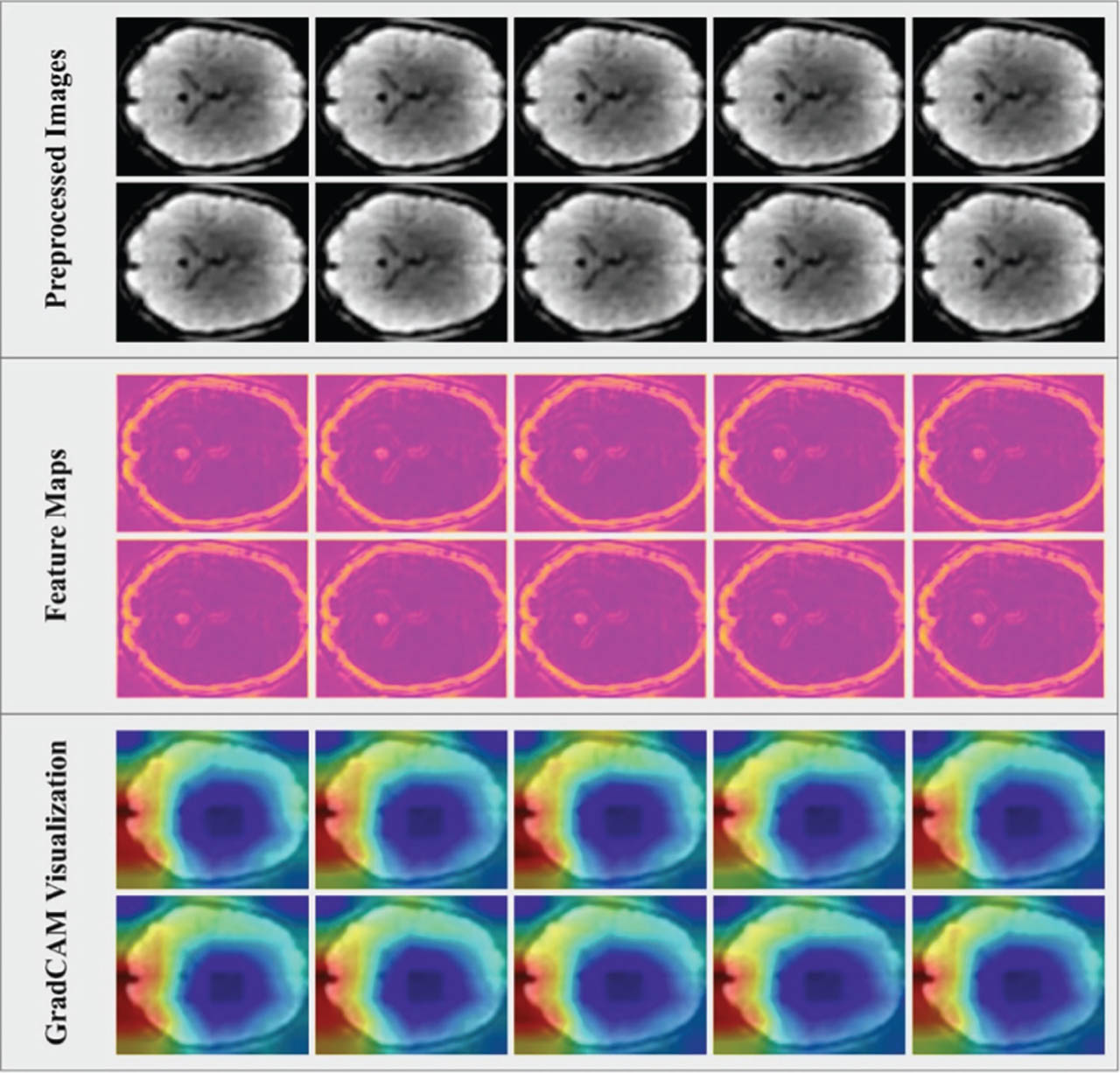
Figure 4:
Preprocessed images, feature maps, and GradCAM visualizations.
b. Assessment criteria
The performance evaluation measures are vital to know how fine a method is executing on testing data. The performance measure used in this study are as follows:
b.i. Accuracy
Accuracy is a standard performance metric defined as the ratio of correctly predicted samples to the total number of samples, where correct predictions include both true positives (TPs) and true negatives (TNs). It is defined as single significant measure when assessing classifier methods. It is the portion of predictions acquired by the method. It is stated below:
Here, TP, TN, FP, and FN represent true positive, true negative, false positive, and false negative, respectively.
b.ii. Precision
Precision is how close the measures are to each other. It is an explanation of random faults and a measure of arithmetical variability. The Eq. (29) is defined as a measure employed where the FP is a concern and not the FN. If a system produces no FPs, then it holds a precision of 1.0.
b.iii. Recall
The recall is a measure employed where the FN out-weighs the FP. It shows how many positive cases are predicted properly with the method. It is formulated below:
b.iv. F measure
This is a harmonic mean of precision and recall. F-Score in (Eq.(31)) displays a united intention of both recall and precision measures. It is greatest when a recall is equivalent to precision. Mainly, when precision is increased, then the recall goes down or else, it goes up.
b.v. MCC
MCC is a correlation coefficient among the true and predicted outcomes that implements well smooth in an case of class imbalance, delivering a value between −1 and +1, while +1 specifies perfect prediction, 0 means a random performance, and −1 indicates wide divergence between prediction and true labels.
c. Result analysis
In this part, the performance VALD of the OADL-MCEDC model is studied under the fMRI dataset for Emotion Recognition dataset. Figure 5 shows the confusion matrices created by the OADL-MCEDC technique with various epochs. The outcomes specify that the OADL-MCEDC approach has effective classification and detection of each class accurately.
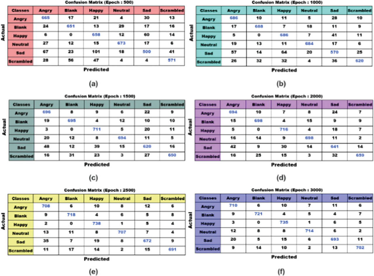
Figure 5:
Confusion matrices of OADL-MCEDC method (A–F) 500–3,000 epochs. OADL-MCEDC, Optimal Attention Deep Learning based Multi-class Emotion Detection and Classification.
Table 2 and Figure 6 represent the emotion recognition of OADL-MCEDC method on several epochs. The outcome indicates that the OADL-MCEDC model properly classified the samples. Under 500 epoch, the proposed OADL-MCEDC approach offers average accury, precin, recall, Fmeasure, and MCC of 94.21%, 82.72%, 82.62%, 82.49%, and 79.15%, respectively. Meanwhile, under 1,500 epochs, the proposed OADL-MCEDC model provides average accury, precin, recall, Fmeasure and MCC of 96.79%, 90.41%, 90.36%, 90.33%, and 88.44%, respectively. In addition, under 3,000 epochs, the proposed OADL-MCEDC techniques offer average accury, Fmeasure, and MCC of 98.33%, 95.02%, 95.00%, 95.00%, and 94.01%, respectively.
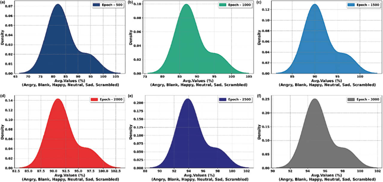
Figure 6:
(A–F) Average outcomes of OADL-MCEDC methodology on numerous epochs. OADL-MCEDC, Optimal Attention Deep Learning based Multi-class Emotion Detection and Classification.
Figure 7 displays the training (TRAN) and VALD accuracy of the OADL-MCEDC system over 3,000 epochs. Both curves gradually rise and slowly converge, which suggests that the technique is learning effectively. The VALD accuracy constantly stays somewhat superior to the TRAN accuracy, implying that the method is not overfitting and generalizes well to unseen data. The fluctuations in accuracy are expected because of the difficulty of the task, but the overall increasing tendency indicates stronger performance and model stability.
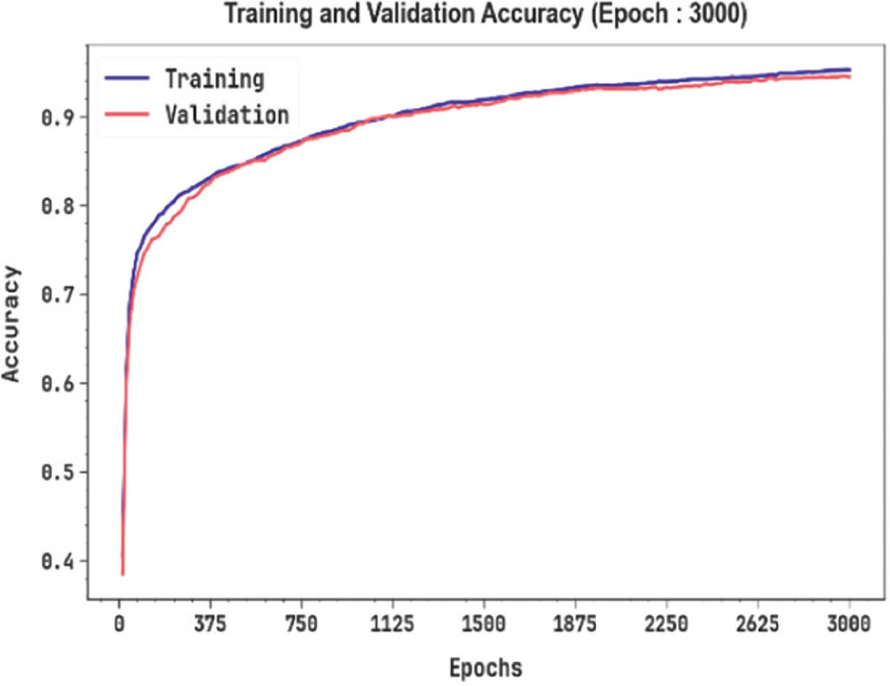
Figure 7:
Accury curve of OADL-MCEDC approach on 3,000 epoch. OADL-MCEDC, Optimal Attention Deep Learning based Multi-class Emotion Detection and Classification.
Figure 8 represents the TRAN and VALD loss of OADL-MCEDC model over 3,000 epochs. Both curves reveal a constant reducing tendency, demonstrating that the model effectively minimizes error throughout learning. The VALD loss stays slightly inferior to the training loss through most epochs, implying good generalization and no signs of overfitting. Even though some fluctuations are monitored become progressively steady and consistent.
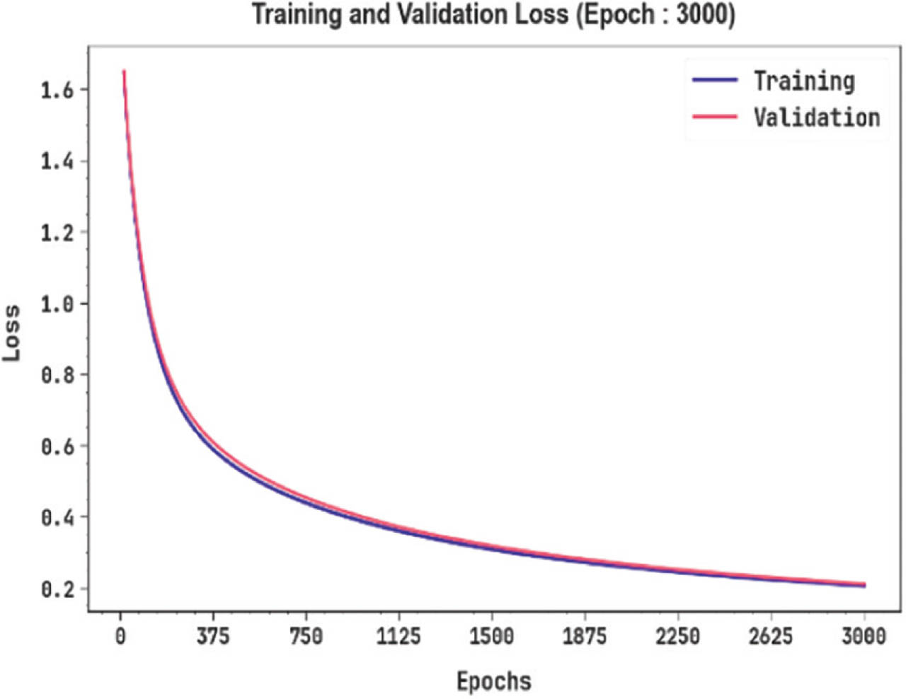
Figure 8:
Loss curve of OADL-MCEDC methodology on 3,000 epoch. OADL-MCEDC, Optimal Attention Deep Learning based Multi-class Emotion Detection and Classification.
Figure 9 represents the precision-recall (PR) curve examination of the OADL-MCEDC model with 3,000 epochs, which gives interpretation into its performance by plotting Precision against Recall for each class. The figure reveals that the OADL-MCEDC technique consistently achieves enhanced PR values across diverse class labels, signifying its capability of maintaining an important portion of TP prediction among all positive predictions (precision) while also taking a huge proportion of actual positives (recall). The stable increases in PR results among all classes depict the efficacy of the OADL-MCEDC model in the classifier procedure.
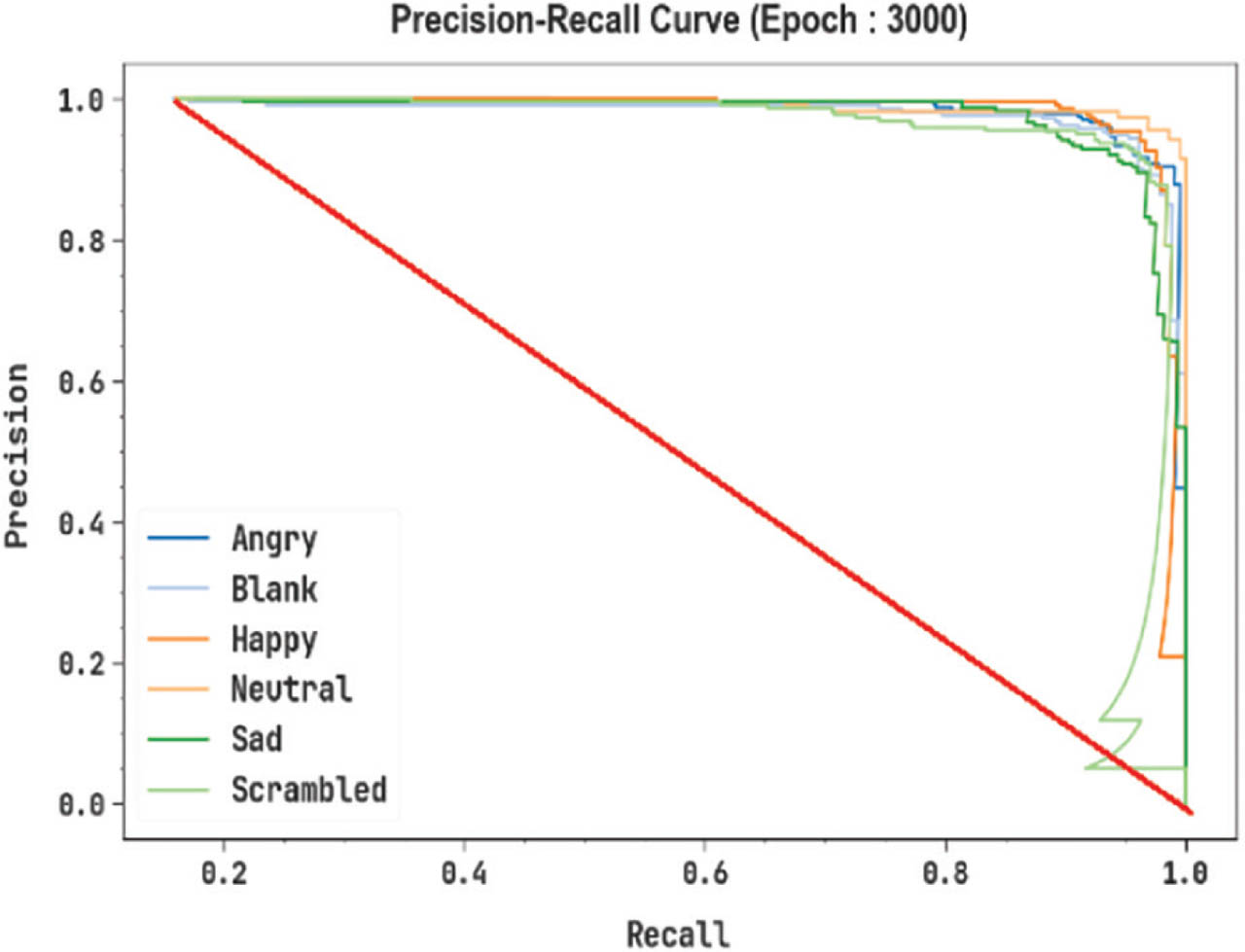
Figure 9:
PR curve of OADL-MCEDC approach on 3,000 epochs. OADL-MCEDC, Optimal Attention Deep Learning based Multi-class Emotion Detection and Classification; PR, precision-recall.
Figure 10 shows the ROC curve of the OADL-MCEDC model being examined. The outcome suggests that the OADL-MCEDC method on 3,000 epochs that achieves improved ROC outcomes across all classes, indicating an important ability to distinguish the classes. This constant tendency of enhanced ROC values across several classes implies the efficacious operations of the OADL-MCEDC model in predicting classes, emphasizing the strong nature under the classifier procedure.
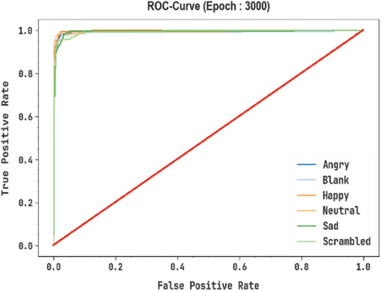
Figure 10:
ROC curve of OADL-MCEDC system on 3,000 epoch. OADL-MCEDC, Optimal Attention Deep Learning based Multi-class Emotion Detection and Classification.
The comparative analysis of OADL-MCEDC approach with existing systems is shown in Table 4 and Figure 11 [33, 34]. The simulation results stated that the OADL-MCEDC approach outperformed better performances. Depends on accury, the pro-posed OADL-MCEDC approach has obtained higher outcomes with accury of 98.33% whereas the random forest (RF) of 91.00%, 1D CNN of 87.00%, DNN of 87.34% attains moderately superior values, respectively. In addition, the SVM, Extreme Gradient Boosting (XGBoost), LDA, and DT reach minimal values. Meanwhile, based on precin, the proposed OADL-MCEDC approach has a maximal outcome with precin of 95.02% whereas the LDA of 94.74% and DT of 91.85% accomplish slightly greater outcomes, respectively.
Table 4:
Comparative analysis of OADL-MCEDC methodology with existing approaches
| Approach | Accury | Precin | Recall | Fmeasure |
|---|---|---|---|---|
| 1D CNN | 87.00 | 84.22 | 91.15 | 92.69 |
| SVM | 83.80 | 86.78 | 91.32 | 91.27 |
| XGBoost | 82.00 | 86.60 | 93.34 | 94.09 |
| LDA | 79.00 | 94.74 | 93.09 | 85.75 |
| RF | 91.00 | 83.03 | 84.95 | 93.91 |
| DNN | 87.34 | 85.00 | 92.11 | 93.26 |
| Decision tree | 71.99 | 91.85 | 82.83 | 82.62 |
| OADL-MCEDC | 98.33 | 95.02 | 95.00 | 95.00 |
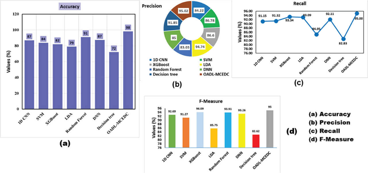
Figure 11:
Comparative analysis of OADL-MCEDC method (A) accury, (B) precin, (C) recall, and (D) Fmeasure. CNN, convolutional neural network; DNN, deep neural network; OADL-MCEDC, Optimal Attention Deep Learning based Multi-class Emotion Detection and Classification; SVM, support vector machine.
The OADL-MCEDC model achieves the highest performance across all metrics, with an accuracy of 98.33%, precision of 95.02%, recall of 95.00%, and F-measure of 95.00%, clearly outperforming the other models. In comparison, the 1D CNN and SVM mod-els perform reasonably well, but they do not reach the level of effectiveness exhibited by OADL-MCEDC. The XGBoost model shows a strong recall, yet its accuracy is still lower than that of OADL-MCEDC. RF and DNN are top performers in terms of accuracy, but they lag behind in both precision and recall compared to OADL-MCEDC.
Furthermore, the 1D CNN, SVM, XGBoost, RF, and DNN techniques gain inferior solutions. Also, based on recall, the proposed OADL-MCEDC approach obtained the highest solution with recall of 95.00% while the DNN of 92.11%, XGBoost of 93.34%, and LDA of 93.09% obtains somewhat higher solutions, correspondingly. Similarly, the 1D CNN, SVM, RF, and DT approaches provide lower performance. At last, based on Fmeasure, the proposed OADL-MCEDC method attains maximal solution with Fmeasure of 95.00%, whereas the RF of 93.91%, DNN of 93.26%, and 1D CNN of 92.69% achieved moderately superior performance, correspondingly. In addition, the SVM, XGBoost, LDA, and DT models obtained lower values. From the detailed outcomes and discussion, it is assured that the OADL-MCEDC technology has proven higher performance over other models. The OADL-MCEDC model's complexity, due to its hybrid capsule network and Attention-BiLSTM, demands significant computational resources. The Nadam optimizer improves convergence efficiency, ensuring reduced training time. The model's computational efficiency is further enhanced by focusing on relevant brain regions, minimizing redundant computations. The model is robust against noise and variability in fMRI signals, thanks to preprocessing techniques such as motion correction and noise filtering. The hybrid capsule network preserves key spatial patterns, and the attention mechanism highlights important temporal features, ensuring reliable performance.
V. Conclusion
This article introduced an OADL-MCEDC framework on fMRI Images, which utilizes an attention-based DL architecture to classify human emotions from fMRI images. To accomplish that, the presented OADL-MCEDC methodology primarily preprocessed the input images utilizing motion correction, spatial normalization, slice-timing correction, and noise filtering techniques, guaranteeing high-quality and consistent fMRI inputs. These preprocessed fMRI images are further transformed into feature maps for deep analysis. To achieve effective feature representation, a hybrid capsule network is used to extract discriminative patterns crucial for ED. Following that, an Attention-BiLSTM network is designed for effective classification of six emotional states: angry, blank, happy, neutral, sad, and scrambled. Lastly, the Nadam optimizer is integrated for optimal fine-tuning, ensuring better model stability and performance. Comprehensive simulation studies are performed to demonstrate the superiority of the OADL-MCEDC methodology. The comparative analysis highlighted improvements in the OADL-MCEDC technique over other state-of-the-art methods across multiple evaluation measures. The described model is likely to find its practical application in both clinical and technological spheres. For instance, using the described model in the diagnosis of mental conditions, physicians will be able to determine affective disorders such as depression, anxiety, and emotional instability through the analysis of activity patterns of the brain using fMRI. Furthermore, the described model can help develop new brain-computer inter-face systems that rely on ED (from neurons' received signals). It should be noted that this technology can be helpful when creating human-machine interfaces to enhance interaction between disabled people and devices controlled by brain signals. Thus, ED can be helpful not only in terms of diagnosing patients but also in improving their quality of life.
Future work will focus on validating the proposed OADL-MCEDC framework on larger and more diverse fMRI datasets to further evaluate its generalizability and robustness across different subjects and experimental conditions.
Abbreviations
- AFER:
Affective Facial Expression Recognition
- AI:
Artificial Intelligence
- BART:
Bidirectional and Auto-Regressive Transformers
- Bi-LSTM:
Bidirectional Long Short-Term Memory
- CLIP:
Contrastive Language–Image Pre-training
- DPMN:
Dual-Polarity Memory Network
- DR:
Dimension Reduction
- DT:
Decision Tree
- DWT:
Discrete Wavelet Transform
- FER:
Facial Expression Recognition
- GAT:
Graph Attention Network
- GLCM:
Gray-Level Co-occurrence Matrix
- GradCAM:
Gradient-weighted Class Activation Mapping
- IEC:
Imaging Emotion Classification
- IER:
Image Emotion Recognition
- KNN:
K-Nearest Neighbors
- LBP:
Local Binary Pattern
- LDA:
Linear Discriminant Analysis
- LSTM:
Long Short-Term Memory
- ML:
Machine Learning
- ReLU:
Rectified Linear Unit
- ROC:
Receiver Operating Characteristic
- ROIs:
Regions of Interest
- RPN:
Region Proposal Network
- ViT:
Vision Transformer
Notes
[5] Contributed by Author's Contributions
L. Dinesh is responsible for designing the framework, analyzing the performance, validating the results, and writing the article. G. Indirani is responsible for collecting the information required for the framework, providing software, critical review, and administering the process.
[7] Data Availability Statement
The data that support the findings of this study are openly available in Kaggle repository at https://www.kaggle.com/datasets/irajahangari/fmri-data-set-for-emotionrecognition, reference number [31].