
Representative works—key advantages & disadvantages
| Reference | Core idea | Advantages | Limitations |
|---|---|---|---|
| [1] | CNN encoder + RNN decoder end-to-end image→sentence | Simple, effective end-to-end learning; good baseline for fluency. | Limited visual grounding (global CNN features); often produces generic captions and can miss fine details. |
| [2] | Deep vision–language architectures used in natural images can be effectively adapted to remote sensing | Effective feature extraction for remote sensing images. Improved natural-language description generation. Reduced dependence on manual annotation. | Lack of attention mechanisms. Dataset constraints. No multimodal fusion enhancements. Not benchmarking against state-of-the-art models. |
| [3] | Uses object-level region features (bottom–up) + top–down attention controller | Stronger grounding to objects; better fine-grained descriptions and improved metrics; became standard input for many models. | Requires object detector pretraining (computational and annotation cost); detector biases affect captions. |
| [4] | RL-based sequence-level training optimizing CIDEr and other metrics | Directly optimizes evaluation metrics, leading to large empirical improvements; reduces train–test objective mismatch. | RL training can be unstable; can encourage metric-specific artifacts (over fitting to metric quirks). |
| [5] | Adds spatial attention over CNN feature maps during decoding | Improved relevance; produces interpretable attention maps; better at localizing salient regions while generating words. | Attention over grid features is still coarse; struggles with object identity and fine relations. |
| [6] | Multi-level transformer encoder + mesh-like decoder memory for better cross-level fusion | Exploits low- and high-level features simultaneously; strong performance with a fully attentive architecture; captures relations better. | More complex architecture and heavier compute; may need careful tuning and larger data. |
| [7] | Pretraining on image–text pairs using object tags as anchor tokens | Strong cross-modal representations; excellent transfer to captioning and V + L tasks; reduces need for task-specific data. | Large-scale pretraining is compute- and data-intensive; it relies on detector-generated object tags (propagates detector errors). |
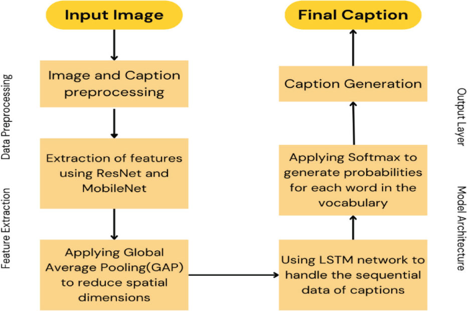
Figure 1:
Proposed hybrid architecture model. GAP, global average pooling; LSTM, long short-term memory.
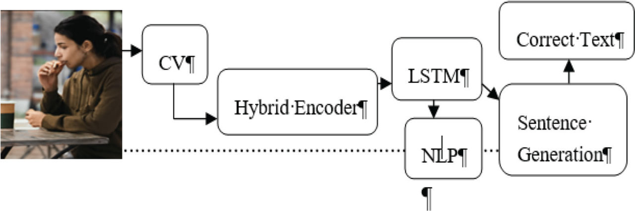
Figure 2:
An illustration of a multimodal IC network. CV, computer vision; IC, image captioning; LSTM, long short-term memory.
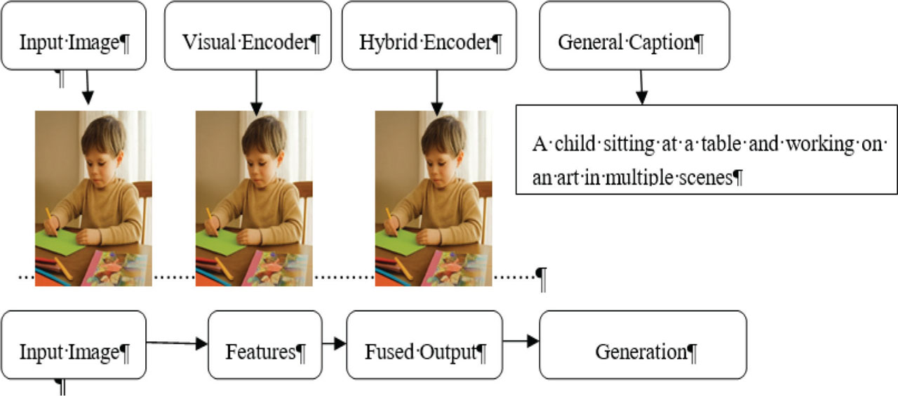
Figure 3:
Dense captioning explanation numerous annotations with individual forward pass.
Table 1:
Obtained outcome from the individual DL model along with hybrid model
| Model name | BLUE-1 | BLUE-2 | Trainable parameters | Non-trainable parameters |
|---|---|---|---|---|
| VGG-19 | 0.87524 | 0.81234 | 139,570,240 | 0 |
| VGG-16 | 0.85432 | 0.79648 | 118,684,640 | 0 |
| ResNet50 | 0.84657 | 0.78543 | 4,231,976 | 19,888 |
| MobileNet | 0.83636 | 0.75032 | 705,330 | 3,314 |
| Dense Net | 0.81564 | 0.75546 | 1,410,664 | 6,630 |
| InceptionV3 | 0.79654 | 0.71542 | 3,526,650 | 15,670 |
| Proposed hybrid architecture | 0.98426 | 0.90558 | 5,204,864 | 33,428 |
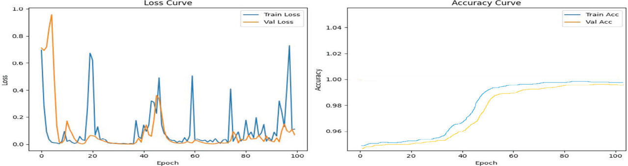
Figure 4:
Accuracy & loss curve of proposed hybrid architecture model for epoc 100.
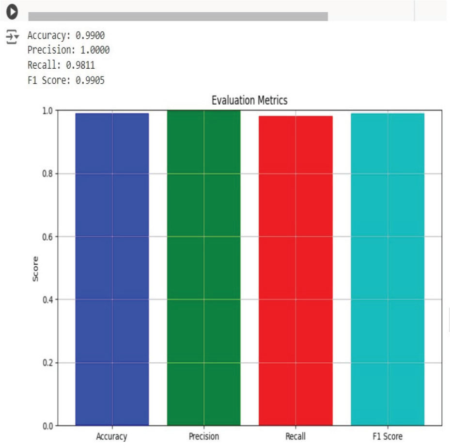
Figure 5:
Evaluation metrics.
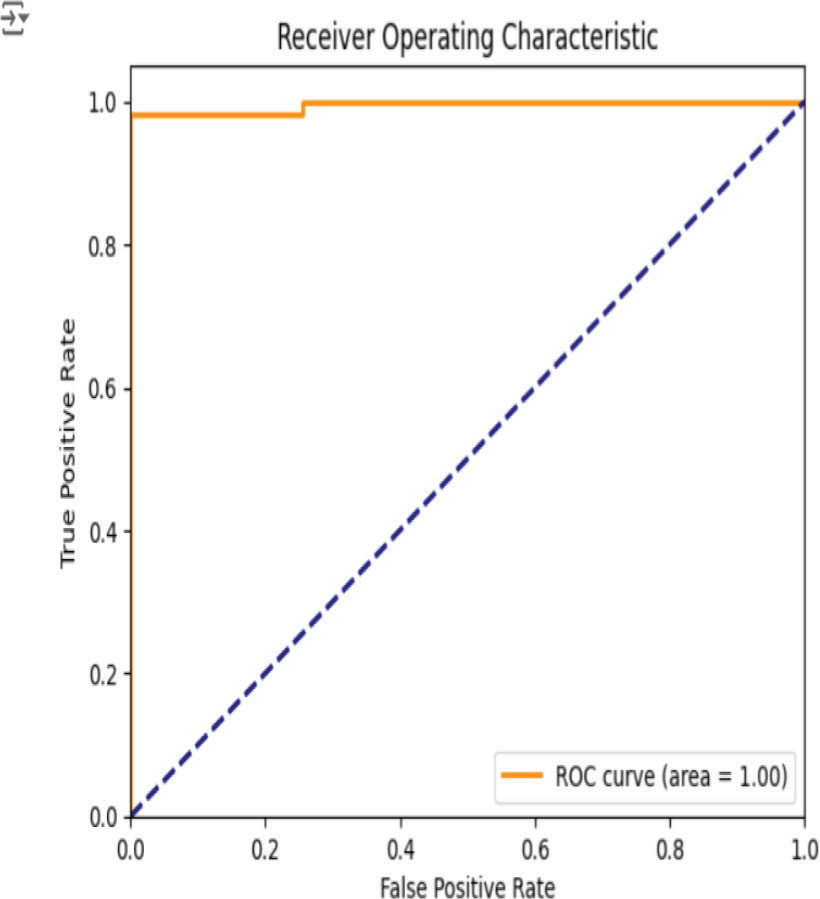
Figure 6:
ROC curve. ROC, receiver operating characteristic.
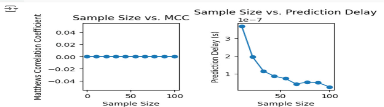
Figure 7:
Sample size vs. MCC and sample size vs. prediction delay.
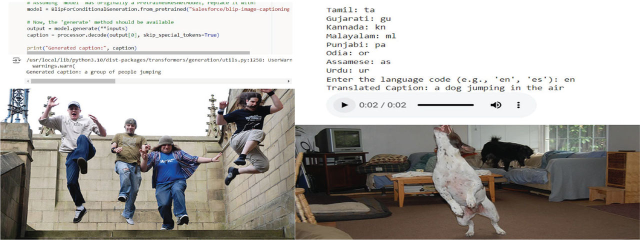
Figure 8:
Sample output.
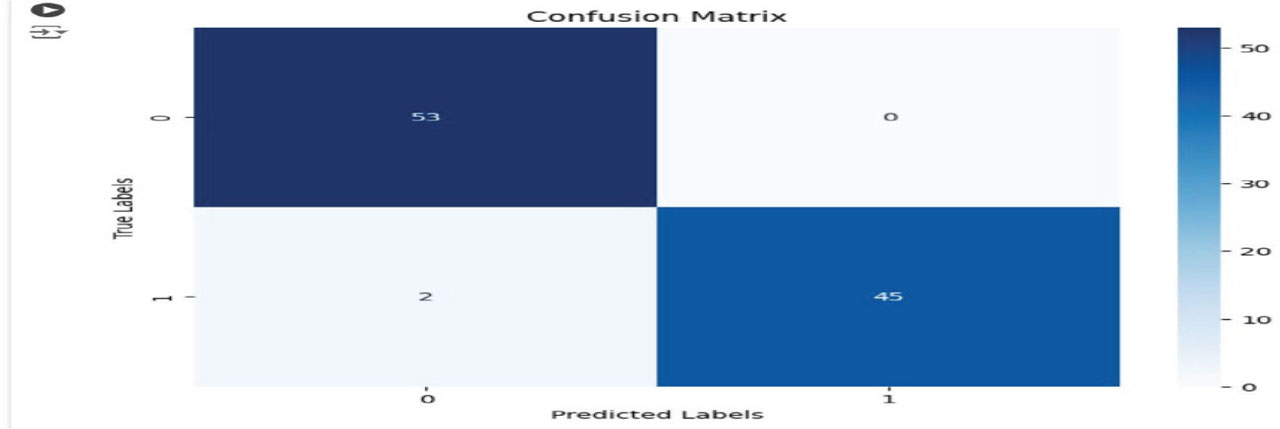
Figure 9:
Confusion matrix.
Table 2:
Paired samples statistics (T-test)
| Mean | N | Std. deviation | Std. error mean | ||
|---|---|---|---|---|---|
| Pair 1 | HybridModel_BLEU | 0.1927 | 1,999 | 0.18642 | 0.01874 |
| MobileNetV2_BLEU | 0.0000 | 1,999 | 0.00005 | 0.00000 |
Table 3:
Paired samples correlations
| N | Correlation | One-sided p | Two-sided p | ||
|---|---|---|---|---|---|
| Pair 1 | HybridModel_BLEU & MobileNetV2_BLEU | 2 | 0.091 | 0.186 | 0.372 |
| 1,999 |
Table 4:
Paired samples test
| Mean | Std. deviation | Std. error mean | Lower | ||
|---|---|---|---|---|---|
| Pair 1 | HybridModel_BLEU – MobileNetV2_BLEU | 0.192 | 0.18641 | 0.01874 | 0.15553 |
Table 5:
Paired samples test
| Upper | t | df | One-sided p | Two-sided p | ||
|---|---|---|---|---|---|---|
| Pair 1 | HybridModel_BLEU – MobileNetV2_BLEU | 0.22989 | 10.286 | 98 | <0.001 | <0.001 |
Table 6:
Paired samples effect sizes
| Standardizera | V point estimate | Lower | |||
|---|---|---|---|---|---|
| Pair 1 | HybridModel_BLEU – MobileNetV2_BLEU | Cohen’s d | 0.18641 | 1.034 | 0.788 |
| Hedges’ correction | 0.18786 | 1.026 | 0.782 |
Table 7:
Paired samples effect sizes
| Upper | |||
|---|---|---|---|
| Pair 1 | HybridModel_BLEU – MobileNetV2_BLEU | Cohen’s d | 1.276 |
| Hedges’ correction | 1.267 |
Table 8:
Npar tests (Wilcoxon signed ranks test) ranks
| N | Mean rank | Sum of ranks | ||
|---|---|---|---|---|
| HybridModel_BLEU – MobileNetV2_BLEU | Negative ranks | 1797a | 49.00 | 4753.00 |
| Positive ranks | 0b | 0.00 | 0.00 | |
| Ties | 202c | |||
| Total | 1999 |
Table 10:
Ablation results (BLEU scores)
| Model variant | Fusion | GAP | BLEU-1 | BLEU-2 | BLEU-3 | BLEU-4 |
|---|---|---|---|---|---|---|
| MobileNet | – | Yes | 0.836 | 0.750 | 0.664 | 0.521 |
| ResNet50 | – | Yes | 0.846 | 0.785 | 0.691 | 0.552 |
| ResNet50 + MobileNet | Addition | Yes | 0.912 | 0.843 | 0.731 | 0.584 |
| ResNet50 + MobileNet | Concatenation | Yes | 0.984 | 0.872 | 0.721 | 0.592 |
| ResNet50 + MobileNet | Concatenation | No (Flatten) | 0.927 | 0.861 | 0.702 | 0.556 |
Table 11:
Comparative accuracy for considering different papers
| Reference | Database | Accuracy obtained |
|---|---|---|
| [1] | Flickr 30k | For BLEU-1: 0.72 |
| For BLEU-2: 0.63 | ||
| For BLEU-3: 0.51 | ||
| For BLEU-4: 0.38 | ||
| [2] | Remote sensing image captioning dataset | ForBLEU-1: 0.661 |
| For BLEU-2: 0.476 | ||
| For BLEU-3: 0.375 | ||
| For BLEU-4: 0.302 | ||
| [8] | Flickr 8k | 0.45 (20 Epoch) and |
| 0.73 (50 Epoch) | ||
| [11] | Flickr 8k | For BLEU-1: 0.28 |
| For BLEU-2: 0.17 | ||
| For BLEU-3: 0.08 | ||
| For BLEU-4: 0.02 | ||
| [12] | Flickr8k | For BLEU-1: 0.31 |
| For BLEU-2: 0.10 | ||
| For BLEU-3: 0.04 | ||
| For BLEU-4: 0.02 | ||
| [18] | Flickr 8k | For BLEU-1: 0.76 |
| For BLEU-2: 0.74 | ||
| For BLEU-3: 0.73 | ||
| For BLEU-4: 0.72 | ||
| [19] | Flickr 8k | For BLEU-1: 0.75 |
| For BLEU-2: 0.61 | ||
| For BLEU-3: 0.47 | ||
| For BLEU-4: 0.32 | ||
| [22] | Flickr 8k | For BLEU-1: 0.74 |
| For BLEU-2: 0.65 | ||
| For BLEU-3: 0.49 | ||
| For BLEU-4: 0.31 | ||
| Proposed approach | Flickr 8k and Flickr30k | For BLEU-1: 0.98 |
| For BLEU-2: 0.87 | ||
| For BLEU-3: 0.72 | ||
| For BLEU-4: 0.59 |