
I. Introduction
Recently, the electricity consumption in residential buildings has become more complex due to the penetration of renewable energy, such as solar panels, and the increased use of electrical appliances resulting in a significant increase in household power consumption. [1]. In such systems, predicting home energy consumption plays a critical role in home energy management, where it can be used for load scheduling, improving energy efficiency, and reducing carbon emissions. An accurate prediction model allows effective control of home appliances and energy resources. It plays a key role as an input to the home energy management system (HEMS) for energy optimization [2, 3].
Basically, the load prediction can be divided into four categories, with respect to the time horizons [1, 4]:
Very-short-term load forecasting (VSTLF): Power is predicted over a range of 1 min to 1 hr, making it suitable for fast response and real-time operation.
Short-term load forecasting (STLF): Power is predicted over a range of 1 hr to 1 week, making it suitable for short-term planning and daily operation.
Medium-term load forecasting (MTLF): Power is predicted over a range of 1 week to 1 year, making it suitable for medium-term planning and seasonal load adjustment.
Long-term load forecasting (LTLF): Power is predicted beyond 1 year, for long-term and strategic planning.
The short-term home appliance energy consumption prediction was proposed in [4], where time intervals of 10 min and 15 min were used for 1-day-ahead prediction. The work in [5] used a 15-min time interval. In [6], 1-hr data was used to predict the next 1-hr energy consumption. The hourly and daily energy consumptions of the residential buildings were proposed in [7]. The residential load predictions for 6-hr, 12-hr, and 24-hr time horizons were proposed in [8]. In [9, 10], the performances of household energy consumption predictions under different time horizons: VSTLF (every hour), STLF (every day and week), and MTLF (every month and quarter) were studied.
Recently, most studies have employed machine learning techniques to predict household energy consumption. Prediction techniques can be divided into four major categories: statistical models, traditional machine learning-based methods (including tree-based methods), deep learning-based methods, and hybrid or ensemble approaches. The artificial neural network (ANN) improved with the behavior model was proposed to predict the next day’s hourly energy consumption [11]. The combination of weather and power data was used to train the ANN to predict the power consumption [12]. The traditional and deep learning-based machine learning techniques were employed to predict the appliances and total power consumption by considering the weather data [13].
The long short-term memory (LSTM), a powerful deep learning method for handling time-series data, is widely used in energy consumption prediction. In [14], the LSTM was employed to predict the energy consumption of the common home appliances in the HEMS. The multivariate LSTM that integrates the weather features was proposed in [15]. The load prediction was improved by integrating the LSTM with human behavior recognition [16]. The LSTM was used to predict appliance energy based on temperature, humidity, wind speed, dew point, and weight factors [17]. A cloud-assisted deep learning model using multi-attribute convolutional long short-term memory was proposed to predict short-term energy consumption drawn by home appliances [18].
The LSTM, recurrent neural network (RNN), and gated recurrent unit (GRU) were employed to predict the energy consumption and environment parameters [19]. The combination of convolutional neural network (CNN) and LSTM was used to improve home consumption prediction accuracy [20], where the CNN was used to extract spatial features, while the LSTM was used to extract temporal features. The integration of CNN with a BiLSTM and an attention mechanism was proposed in [21] to improve the energy consumption model’s handling of spatial and temporal features.
In [22], the energy consumption models ensembled the three statistical predictions, namely auto regressive moving average, auto regressive integrated moving average (ARIMA), and seasonal ARIMA (SARIMA) with ANN to improve the prediction accuracy. The fusion of statistical prediction, seasonal autoregressive integrated moving average with exogenous variables (SARIMAX) and machine learning techniques (random forest [RF], LSTM, extreme gradient boosting [XGB]) were employed to predict the energy load accurately [23] by utilizing the SARIMAX for dealing with time-series trends, RF and XGB for capturing non-linearity, and LSTM for capturing temporal dependencies.
Although many studies have examined residential energy consumption extensively, only a limited number explicitly discusses the detailed appliance usage information, despite its dominant influence on residential load variability. Furthermore, no research has yet analyzed the effect of individual load power consumption on the accuracy of predicting total power consumption. This research addresses these gaps by proposing a prediction framework that exposes both individual appliance and total power consumptions, and the impact on improving the prediction accuracy. To provide a comprehensive study, the comparisons of multi-horizon predictions and different machine learning methods are investigated.
The main contributions of the proposed approach are:
It considers both individual appliance power consumption prediction and total power prediction.
It examines the impact of individual appliance power consumption on the prediction performance of total power consumption, where individual appliances are divided into groups based on operational time flexibility for better analysis.
It compares the performance of predictions across the different time horizons: 1 min, 15 min, 1 hr, and 1 day.
It evaluates the performance of tree-based machine learning prediction techniques (RF, light gradient boosting machine [LGBM], XGB), which are suitable for non-sequential data, and deep learning-based prediction techniques (RNN, LSTM, GRU), which are suitable for sequential and time-series data.
The rest of the paper is organized as follows. Section II presents the research method. Section III presents the results and discussion. Section IV covers the conclusion.
II. Research Method
a. Proposed prediction models
The architectures of the proposed models are illustrated in Figures 1–5. It consists of five schemas with respect to the types of power prediction and input feature groups, as follows:
Scheme-1: The individual appliance power prediction.
Scheme-2: Total power prediction with Feature Group-A (water heater [WH] power, washing machine [WM] power, rice cooker [RC] power, microwave oven [MO] power, total power).
Scheme-3: Total power prediction with Feature Group-B (refrigerator [RFG] power, freezer [FZ] power, water pump [WP] power, lighting [LG] power, total power).
Scheme-4: Total power prediction with Feature Group-C (water heater power, washing machine power, RC power, MO power, RFZ power, FZ power, WP power, lighting power, total power).
Scheme-5: Total power prediction with Feature Group-D (total power).
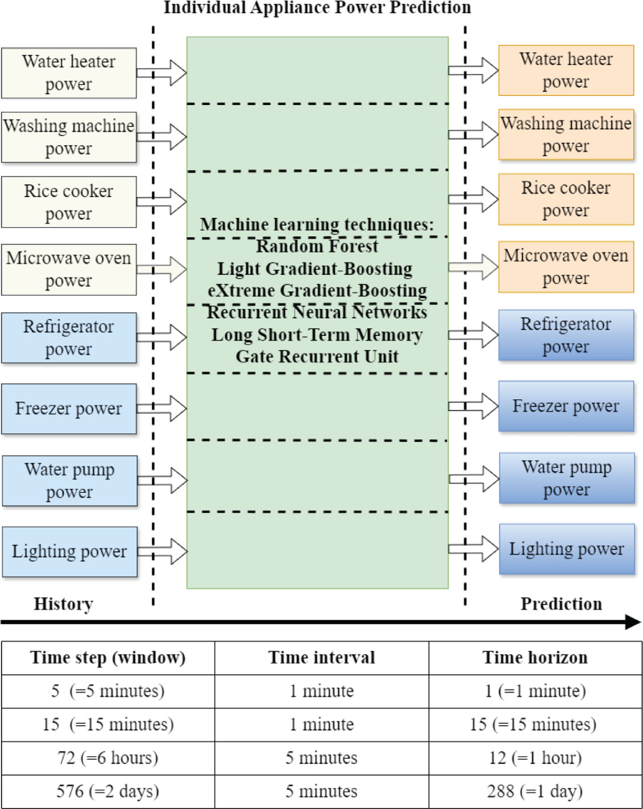
Figure 1:
Architecture of Scheme-1. GRU, gated recurrent unit; LGBM, light gradient boosting machine; LSTM, long short-term memory; RF, random forest; RNN, recurrent neural network; XGB, extreme gradient boosting.
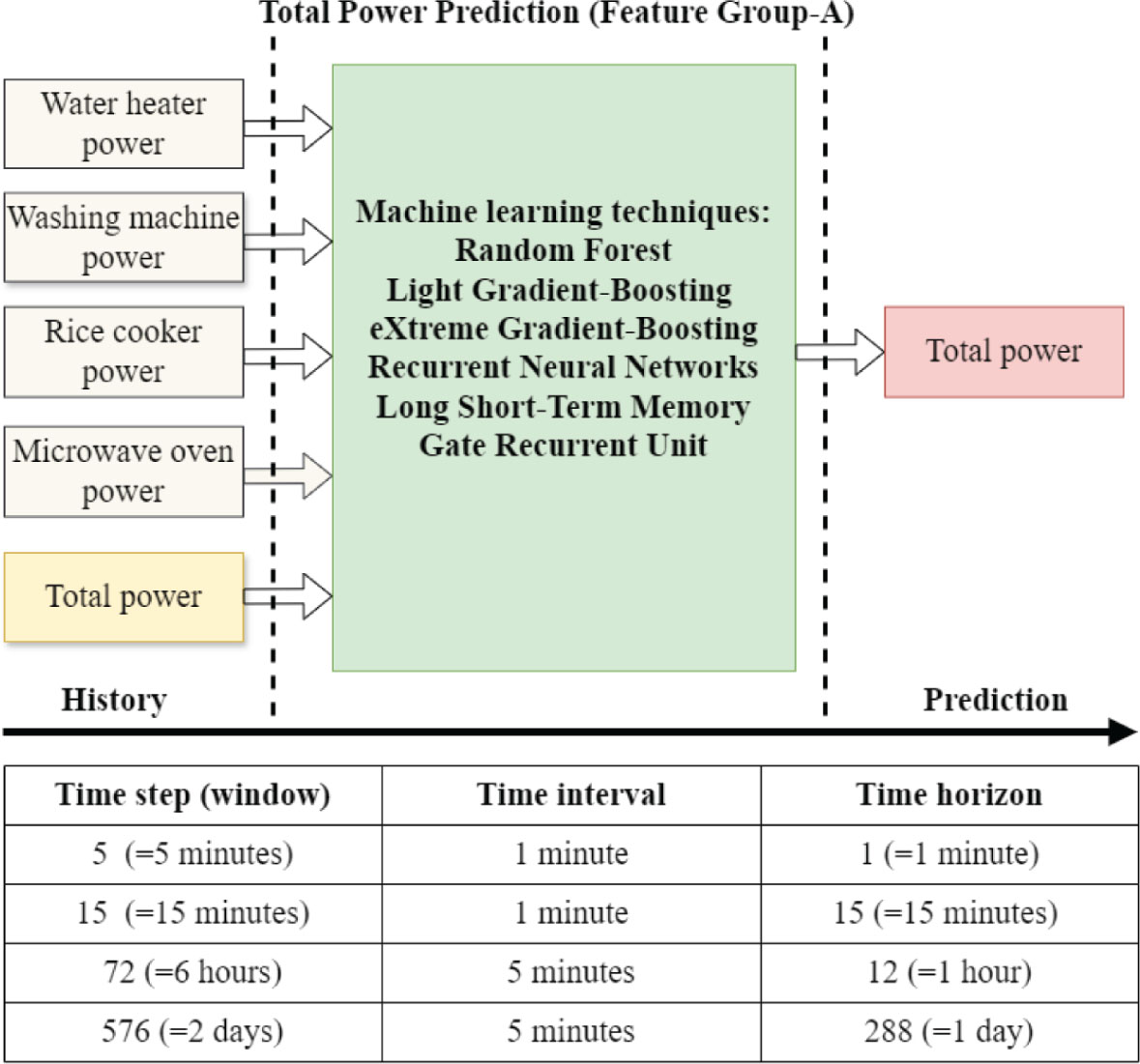
Figure 2:
Architecture of Scheme-2. GRU, gated recurrent unit; LGBM, light gradient boosting machine; LSTM, long short-term memory; RF, random forest; RNN, recurrent neural network; XGB, extreme gradient boosting.
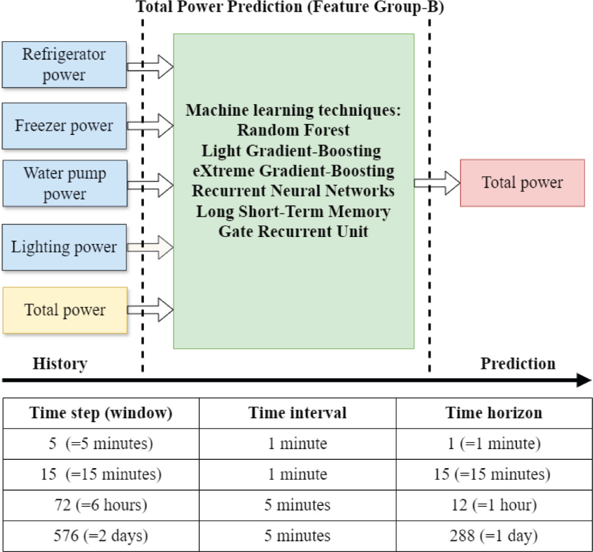
Figure 3:
Architecture of Scheme-3. GRU, gated recurrent unit; LGBM, light gradient boosting machine; LSTM, long short-term memory; RF, random forest; RNN, recurrent neural network; XGB, extreme gradient boosting.
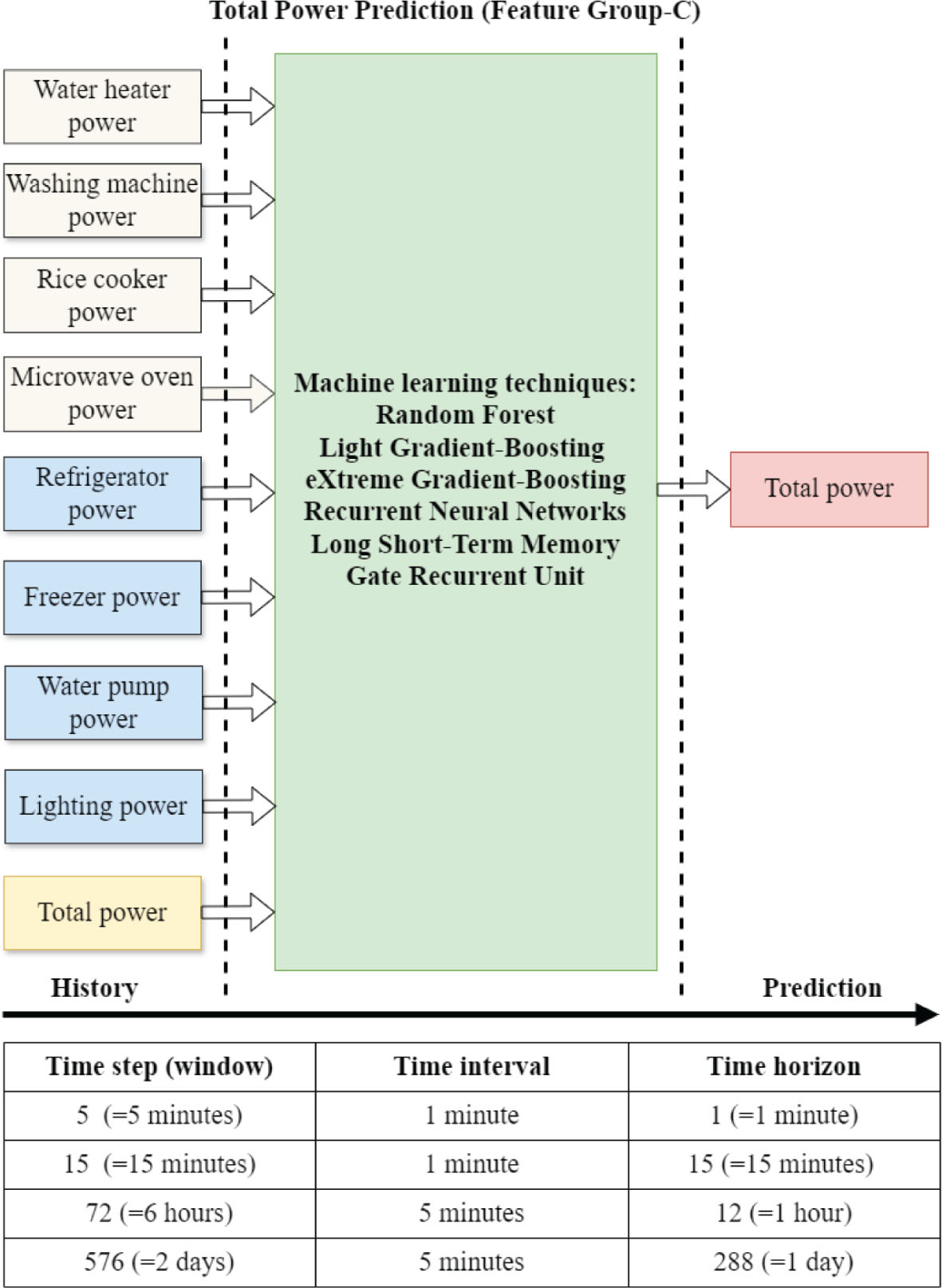
Figure 4:
Architecture of Scheme-4. GRU, gated recurrent unit; LGBM, light gradient boosting machine; LSTM, long short-term memory; RF, random forest; RNN, recurrent neural network; XGB, extreme gradient boosting.
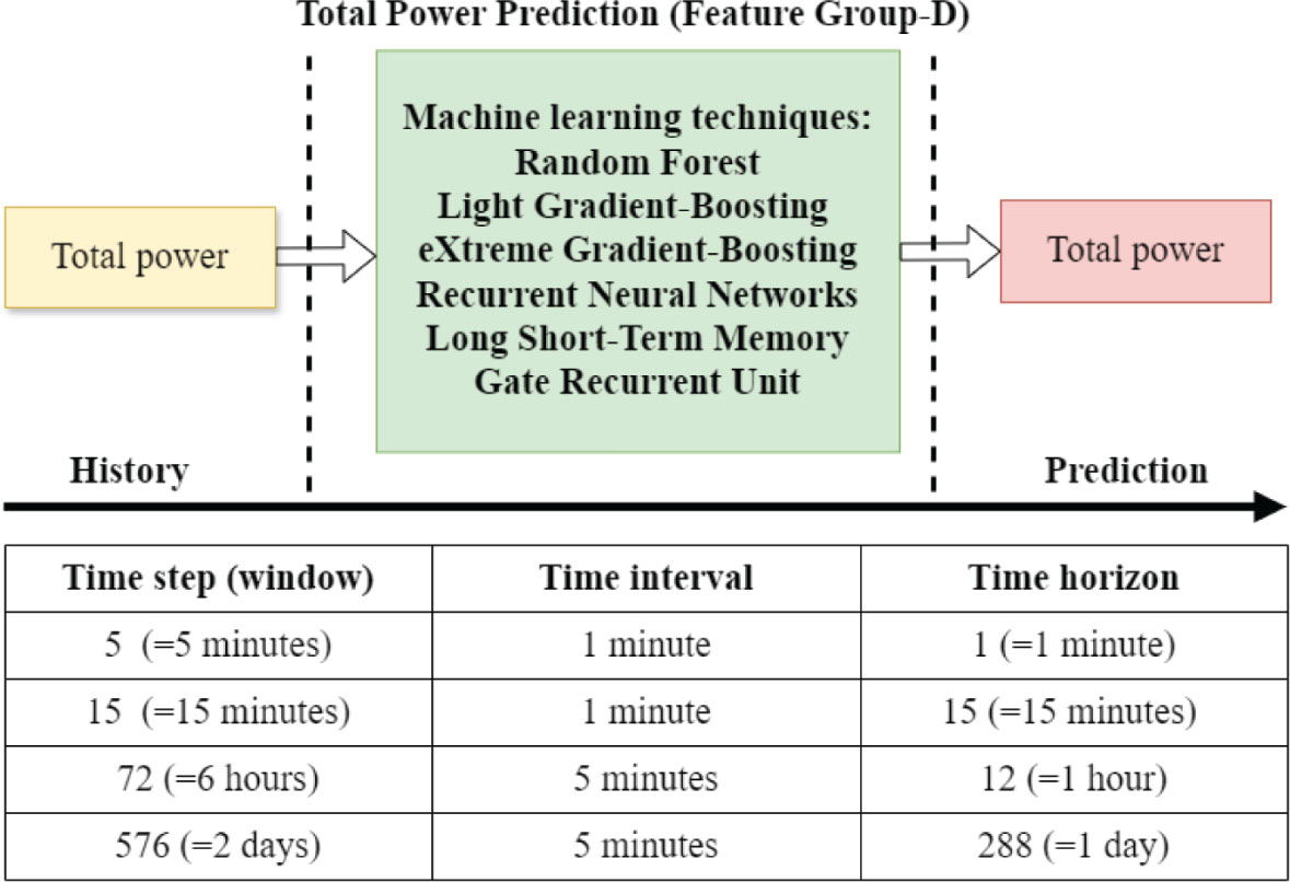
Figure 5:
Architecture of Scheme-5. GRU, gated recurrent unit; LGBM, light gradient boosting machine; LSTM, long short-term memory; RF, random forest; RNN, recurrent neural network; XGB, extreme gradient boosting.
Scheme-1 is used to predict the individual appliance power at a future time based on its previous time power consumption. In this work, eight home appliances are considered, namely water heater, washing machine, rice cooker, MO, refrigerator, freezer, WP, and lighting. It is worth noting that with the recent development of IoT technology, individual appliance power consumption monitoring can be implemented easily, as developed in [24, 25].
Scheme-2 to Scheme-5 is used to predict the total power at a future time based on the different input features at previous times. Scheme-2 uses Feature Group-A, consisting of the reschedulable loads WH power, WM power, RC power, MO power and the total power, as the input features. The reschedulable load is the load that the user can control its operating time. Thus, Scheme-2 can be used to examine the impact of occupant behavior when using appliances on the prediction of total power consumption.
Scheme-3 uses Feature Group-B, consisting of the non-reschedulable loads RFG power, FZ power, WP power, LG power and the total power, as the input features. The non-reschedulable load is the load that the user cannot control its operating time. Thus, Scheme-3 can be used to examine the impact of the non-reschedulable appliances on the prediction of total power consumption.
Scheme-4 uses Feature Group-C, consisting of the reschedulable loads, non-reschedulable loads, and the total power, as the input features. Thus, Scheme-4 can be used to examine the impact of all individual appliances on the prediction of total power consumption.
Scheme-5 uses Feature Group-D, consisting solely of total power, as the input feature. Thus, Scheme-5 can be used to examine the performance of total power consumption prediction when using a single feature.
In each scheme, four different time horizons are examined, that is, (a) a 1-min time horizon with a 1-min time interval and a 5-min time step; (b) a 15-min time horizon with a 1-min time interval and a 15-min time step; (c) a 1-hr time horizon with a 5-min time interval and a 6-hr time step; (d) a 1-day time horizon with a 5-min time interval and a 2-day time step. These time-horizon variations fall under VSTLF and STLF. This selection is suitable for analyzing the real-time and hourly or daily operation of home appliances.
As shown in Figures 1–5, six prediction methods are evaluated in each scheme. The prediction techniques are divided into two categories: tree-based machine learning algorithms (RF, LGBM, and XGB) and deep learning-based algorithms (RNN, LSTM, and GRU). The algorithms are described briefly in the following section. The RF, LGBM, and XGB algorithms are usually used for predicting tabular, non-sequential data. Meanwhile, RNNs, LSTMs, and GRUs are commonly used for predicting sequential and time-series data. By evaluating both approaches, the suitability of the algorithm for predicting the short-term power consumption of individual appliances and the total power can be comprehensively analyzed.
b. Tree-based machine learning algorithms
The tree-based machine learning algorithms used in this work are RF, LGBM, and XGB. They are popular and influential tree-based algorithms used for prediction. RF is a tree-based ensemble machine learning technique developed by [26]. It uses trees as the base learners [27] denoted by hj (X,Θj), where X represents the real-value input of predictor, Θj is a collection of random variables. The algorithm is as follows:
Prepare training set TS = {(x1, y1),(x2, y2),...,(xN, yN)}, where xi = (xi.1,..., xi,p)T is the p predictors, and yi is the response;
For j = 1 to J (J is the number of regressors), repeat Step-3 to Step-4;
Pick a bootstrap sample TSj of size N from the training set TS;
Fit a tree using the bootstrapped sample TS:
(a) Start with all observations on a single node
(b) Randomly select the m predictors from the available p predictors
(c) Find the best split from the m predictors
(d) Split the node into two child nodes using the best split
(e) Repeat (b) – (d) until the stopping criterion is met: The prediction of the new point x is given by
The LGBM is a novel gradient boosting machine (GBM) algorithm [28] developed by [29]. It proposes the gradient-based one-side sampling (GOSS) and exclusive feature bundling (EFB) to reduce the computation time. The GOSS reduces the number of samples by focusing on samples with larger gradients and performing random sampling on those with smaller gradients. At first, it sorts the data samples according to the absolute value of the gradients, and selects the highest a × 100% samples. The algorithm then randomly selects b × 100% samples from the rest of data. Finally, the information gain is calculated by amplifying the sampled data with small gradients by a factor . Meanwhile, the EFB is used to bundle exclusive features into a single feature, thus reducing the histogram complexity.
XGB [30] is the most popular implementation of the GBM [31, 32]. The algorithm is briefly described in the following. Suppose the dataset DS with m features and n number of samples is expressed as DS = {(xi, yi) : i = 1,...,n, xi ∈ Rm, yi ∈ R}. The predicted output ŷi of an ensemble tree model is given by
where K is the number of trees, fk denotes the k-th tree, and F is the space of regression trees. The above equation is solved by finding the best set of functions that minimize the following objective function: where I is the loss function, Ω represents the complexity of the model, T is the number of leaf node, ω is the weight of the leaf node, γ and λ are the controlling factors. To optimize the above model Eqs (3) and (4), the model is trained by adding a new function f to minimize the following objective functionThe second-order Taylor polynomial can be used to replace the function ft. Therefore, the objective function becomes
whereThe constant terms in Eq. (6) can be removed to simplify the objective function as follows:
By expanding Ω, the objection function in Eq. (9) can be rewritten as
where Ij is the instance set of leaf j. The optimal weight of leaf j is expressed by and the corresponding optimal values isc. Deep learning-based prediction techniques
The deep learning-based prediction techniques used in this work include RNNs, LSTMs, and GRUs. They are popular prediction algorithms suitable for time-series data. A RNN [33] is a type of ANN in which the output of a neuron is looped back to the same neuron in the next time step. Thus, it can memorize the previous input data. A RNN cell is illustrated in Figure 6, where the hidden layer state at time t (ht) is expressed as
where Whh is the weight matrix for the hidden-to-hidden connection, ht−1 is the hidden layer state at time step t−1, Wxh is the weight matrix for the input to hidden connection, xt is the vector input at time step t, and bt is the bias for the hidden layer.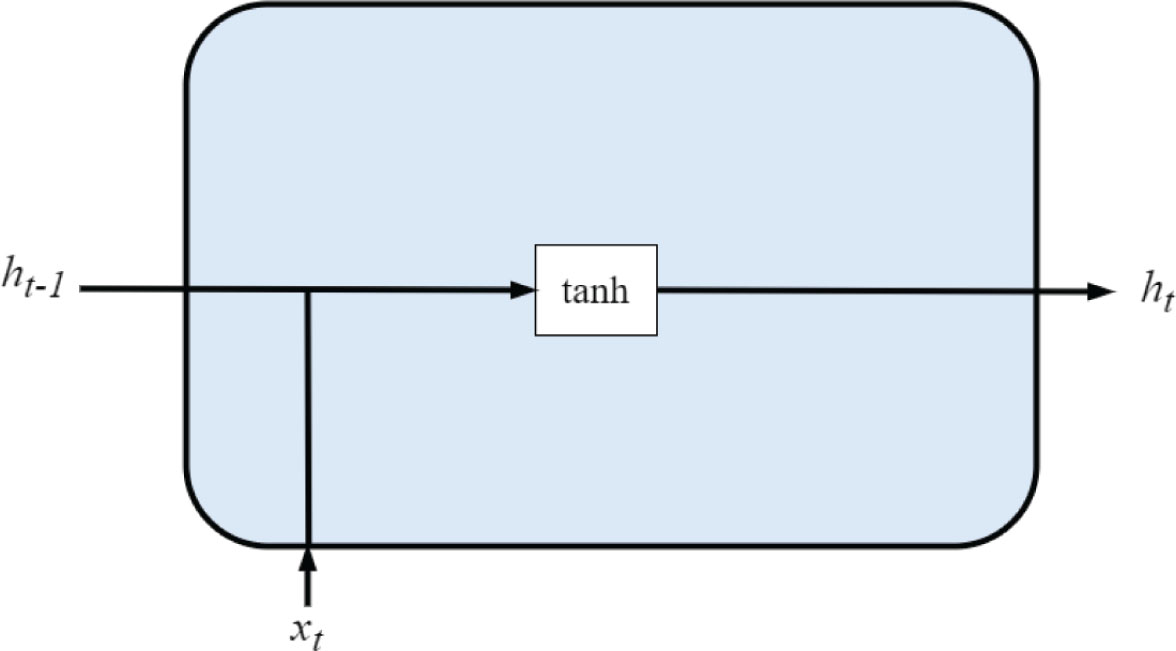
Figure 6:
RNN cell. RNN, recurrent neural network.
The main drawbacks of RNN are the vanishing and exploding gradient problems, in which the gradient becomes too small (vanishing) or too large (exploding). To overcome these problems, the LSTM was proposed by [34]. The LSTM cell is depicted in Figure 7. It consists of an input gate, a forget gate, and an output gate. The input gate is expressed using the following formula:
where σ is a sigmoid function, Wi is the weight matrix for the input gate, bi is the bias for the input gate. The forget gate is expressed using the following formula: where Wf is the weight matrix for the forget gate, bf is the bias for the forget gate. The output gate is expressed using the following formula: where Wo is the weight matrix for the output gate, bo is the bias for the output gate. The cell state is expressed using the following formula: where * indicates the element-wise multiplication, tanh is a hyperbolic tangent function, Wc is the weight matrix for the cell state, bc is the bias for the cell state. The current hidden state is expressed using the following formula: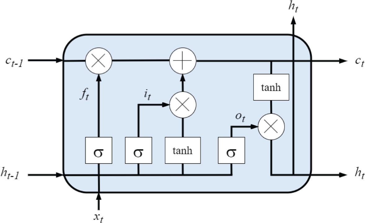
Figure 7:
LSTM cell. LSTM, long short-term memory.
The GRU proposed by [35] is a simplified version of LSTM that improves the performance with less training time. The GRU cell is depicted in Figure 8. The GRU has only two gates, namely the update and reset gates. The update gate is expressed using the following formula:
where Wz is the weight matrix for the update gate. The update gate is expressed using the following formula: where Wr is the weight matrix for the reset gate. The hidden state is expressed using the following function: where Wh is the weight matrix for the hidden state.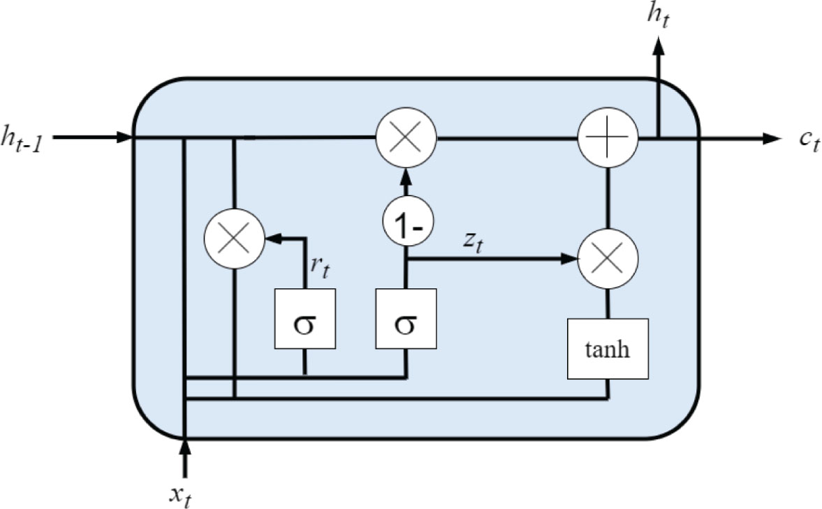
Figure 8:
GRU cell. GRU, gated recurrent unit.
d. Algorithm implementation and evaluation metric
The prediction algorithms are implemented in Python, with machine learning libraries and frame-works employed. The RF is implemented using the scikit-learn library [36]. The LGBM is implemented using the LGBM library [37]. The XGB is implemented using the XGB library [38]. The RNN, LSTM, and GRU are implemented using the Tensorflow framework [39].
The performance of the prediction algorithms are evaluated using two metrics: Normalized mean absolute error (NMAE) and normalized root mean square error (NRMSE). The NMAE and NRMSE are expressed using the following formulas:
where, y, ŷ,n, ymax, ymin are the actual value, the predicted value, the number of samples, the maximum of the actual value, and the minimum of the actual value, respectively.III. Results and Discussion
a. Dataset and machine learning parameters
The dataset was collected from a home using an IoT-based SCADA monitoring system, where individual appliances are measured by smart meters connected to the HMI SCADA wirelessly [25]. The HMI/SCADA system was equipped with local data storage and can be accessed remotely via the internet. It is worth noting that this configuration provided a simple, low-cost home appliance power-monitoring system.
The data were collected over a month, from August 1, 2025 to August 31, 2025, with a 1-min time interval. The dataset consisted of timestamps and power consumption for home appliances (e.g., WH, WM, RC, MO, RFG, FZ, WP, LG), as well as the total power consumption. The dataset is saved in the comma-separated value format. The dataset for 1 month contains 44,637 data points.
To ensure accurate and stable predictions, the dataset is cleaned and preprocessed, including handling missing values, outliers, and normalizing the data to a consistent scale. Then, the data are split into 0.75 for training and 0.25 for testing.
The machine learning parameters used in this work are listed in Table 1 for tree-based algorithms and in Table 2 for deep learning algorithms.
Table 1:
Tree-based machine learning parameters
| RF | LGBM | XGB | |||
|---|---|---|---|---|---|
| Parameter | Value | Parameter | Value | Parameter | Value |
| No. of estimators | 200 | Boosting type | “gbdt” | Booster | “gbtree” |
| Criterion | “Squared error” | No. of leaves | 31 | Min. loss reduction (gamma) | 0 |
| Max. depth | None | Max. depth | −1 | Max. depth | 6 |
| Min. samples split | 2 | Learning rate | 0.05 | Learning rate | 0.05 |
| Min. samples leaf | 1 | No. of estimators | 500 | No. of estimators | 500 |
| Max. features | 1.0 | Objective | “Regression” | Objective | “reg:squarederror” |
| Max. leaf nodes | None | Min. split gain | 0 | Min child weight | 1 |
| Bootstrap | True | Subsample ratio | 0.8 | Subsample ratio | 0.8 |
| Subsample ratio of columns | 0.8 | Subsample ratio of columns | 0.8 | ||
| Regularization alpha | 0 | Regularization alpha | 0 | ||
| Regularization lambda | 0 | Regularization lambda | 1 | ||
Table 2:
Deep learning-based machine learning parameters
| Parameter | Value | ||
|---|---|---|---|
| RNN | LSTM | GRU | |
| No. of units | 64 | 64 | 64 |
| Activation | “tanh” | “tanh” | “tanh” |
| Recurrent activation | - | “Sigmoid” | “Sigmoid” |
| Use bias | True | True | True |
| Kernel initializer | “glorot uniform” | “glorot uniform” | “glorot uniform” |
| Recurrent initializer | “Orthogonal” | “Orthogonal” | “Orthogonal” |
| Bias initializer | “Zeros” | “Zeros” | “Zeros” |
| Input shape | (WINDOW,1) | (WINDOW,1) | (WINDOW,1) |
| Dropout | 0.2 | 0.2 | 0.2 |
| Dense units | 1 | 1 | 1 |
b. Evaluation of individual appliance power prediction
Figures 9–12 depict the NMAE of individual appliance power predictions for 1-min, 15-min, 1-hr, and 1-day time horizons. In each figure, the NMAEs for six methods are compared across eight appliances. To facilitate analysis, the comparison results are summarized in Table 3. Table 3 shows that the lowest NMAE of 0.09% is achieved by the MO using an RNN at a 15-min horizon for reschedulable load, and the lowest NMAE of 0.21% is achieved by the WP using LSTM at a 1-min horizon for non-reschedulable load.
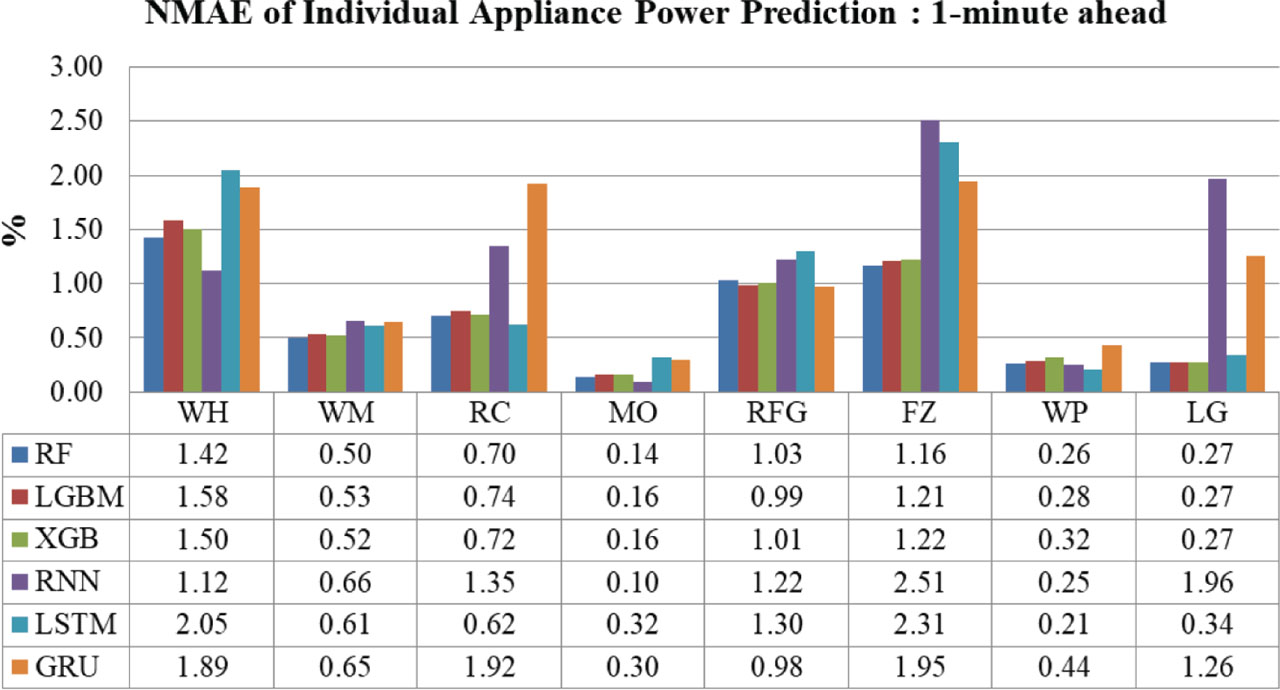
Figure 9:
NMAE of 1-min ahead individual appliance power prediction. GRU, gated recurrent unit; LGBM, light gradient boosting machine; LSTM, long short-term memory; MO, microwave oven; NMAE, normalized mean absolute error; RF, random forest; RNN, recurrent neural network; WP, Water pump; XGB, extreme gradient boosting; FZ, freezer; LG, lighting; RC, rice cooker; RFG, refrigerator; WH, water heater; WM, washing machine.
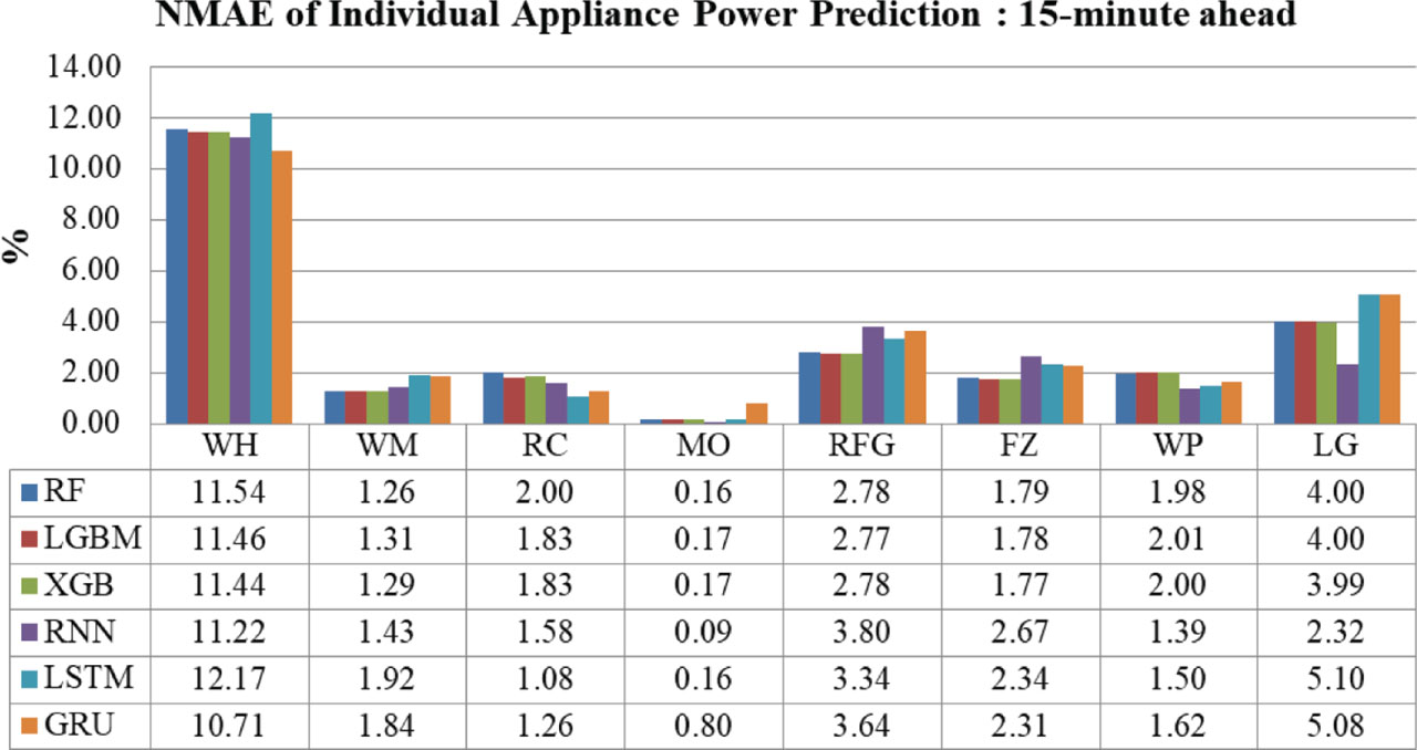
Figure 10:
NMAE of 15-min ahead individual appliance power prediction. GRU, gated recurrent unit; LGBM, light gradient boosting machine; LSTM, long short-term memory; MO, microwave oven; NMAE, normalized mean absolute error; RF, random forest; RNN, recurrent neural network; WP, Water pump; XGB, extreme gradient boosting; FZ, freezer; LG, lighting; RC, rice cooker; RFG, refrigerator; WH, water heater; WM, washing machine.
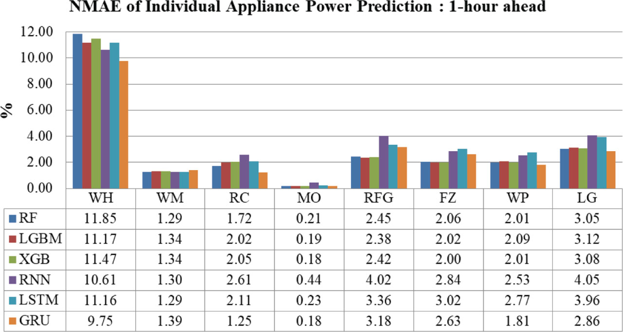
Figure 11:
NMAE of 1-hr ahead individual appliance power prediction. GRU, gated recurrent unit; LGBM, light gradient boosting machine; LSTM, long short-term memory; MO, microwave oven; NMAE, normalized mean absolute error; RF, random forest; RNN, recurrent neural network; WP, Water pump; XGB, extreme gradient boosting; FZ, freezer; LG, lighting; RC, rice cooker; RFG, refrigerator; WH, water heater; WM, washing machine.
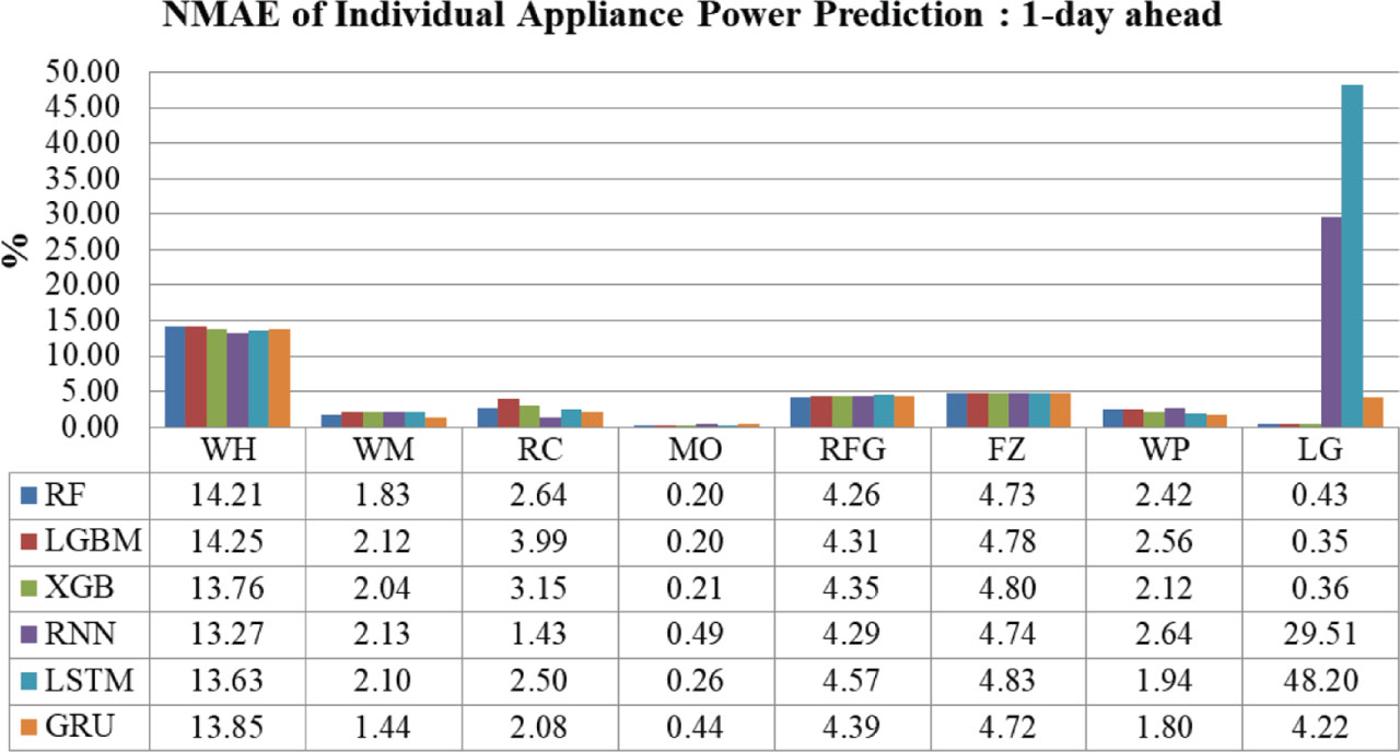
Figure 12:
NMAE of 1-day ahead individual appliance power prediction. GRU, gated recurrent unit; LGBM, light gradient boosting machine; LSTM, long short-term memory; MO, microwave oven; NMAE, normalized mean absolute error; RF, random forest; RNN, recurrent neural network; WP, Water pump; XGB, extreme gradient boosting; FZ, freezer; LG, lighting; RC, rice cooker; RFG, refrigerator; WH, water heater; WM, washing machine.
Table 3:
NMAE comparison of individual appliance power prediction
| Time horizon | Lowest NMAE (%) (appliance, method) | |||
|---|---|---|---|---|
| Reschedulable load | Non-reschedulable load | |||
| Tree-based algorithm | Deep-learning algorithm | Tree-based algorithm | Deep-learning algorithm | |
| 1-min | 0.14 (MO, RF) | 0.10 (MO, RNN) | 0.26 (WP, RF) | 0.21 (WP, LSTM) |
| 15-min | 0.16 (MO, RF) | 0.09 (MO, RNN) | 1.77 (FZ, XGB) | 1.39 (WP, RNN) |
| 1-hr | 0.18 (MO, XGB) | 0.18 (MO, GRU) | 2.00 (FZ, XGB) | 1.81 (WP, GRU) |
| 1-day | 0.20 (MO, RF/LGBM) | 0.26 (MO, LSTM) | 0.35 (LG, LGBM) | 1.80 (WP, GRU) |
Table 3 shows that for reschedulable load, the MO achieves the lowest NMAE for all algorithm types and time horizons. At very short-term prediction, deep learning models outperform tree-based models. It suggests that the MO power usage pattern at short-term time scales shows strong temporal dependence, so it is better captured by temporal-based models such as RNNs. However, at a longer horizon (1-day), the temporal dependency decreases, so that non-temporal models, such as RF or LGBM, outperform temporal-based models.
For the non-reschedulable load, no single appliance achieves the lowest NMAE across all scenarios. For a short-term time horizon, the deep-learning models perform better than tree-based. Interestingly, at a 1-day time horizon, the tree-based model (LGBM) shows the lowest NMAE for LG power prediction. For a stable daily power pattern, such as lighting, a temporal-based model might not exploit it.
Overall comparison in Table 3 indicates that no single prediction algorithm shows superiority across the different appliances and time horizons. Deep learning models perform better for short-term forecasting and for appliances with complex temporal dependencies. Tree-based models perform better at longer time horizons or for appliances with stable usage patterns.
Figures 13–16 depict the NRMSE of individual appliance power predictions for 1-min, 15-min, 1-hr, and 1-day time horizons. Table 4 compares the lowest NRMSEs for individual-appliance power predictions across different scenarios, where the lowest NRMSE of 2.45% is achieved by the MO using an RNN at a 1-min horizon for reschedulable load, and the lowest NRMSE of 3.14% is achieved by the RFG using GRU at a 1-min horizon for non-reschedulable load.
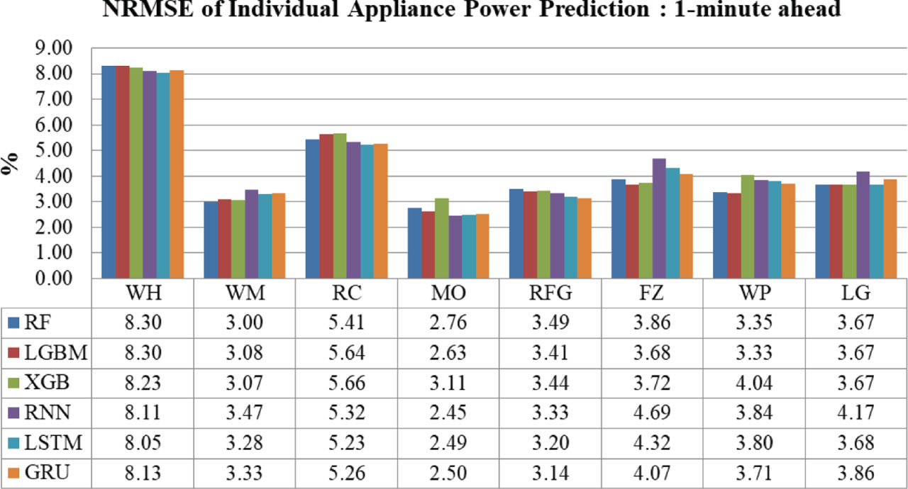
Figure 13:
NRMSE of 1-min ahead individual appliance power prediction. GRU, gated recurrent unit; LGBM, light gradient boosting machine; LSTM, long short-term memory; MO, microwave oven; NRMSE, normalized root mean square error; RF, random forest; RNN, recurrent neural network; WP, Water pump; XGB, extreme gradient boosting; FZ, freezer; LG, lighting; RC, rice cooker; RFG, refrigerator; WH, water heater; WM, washing machine.
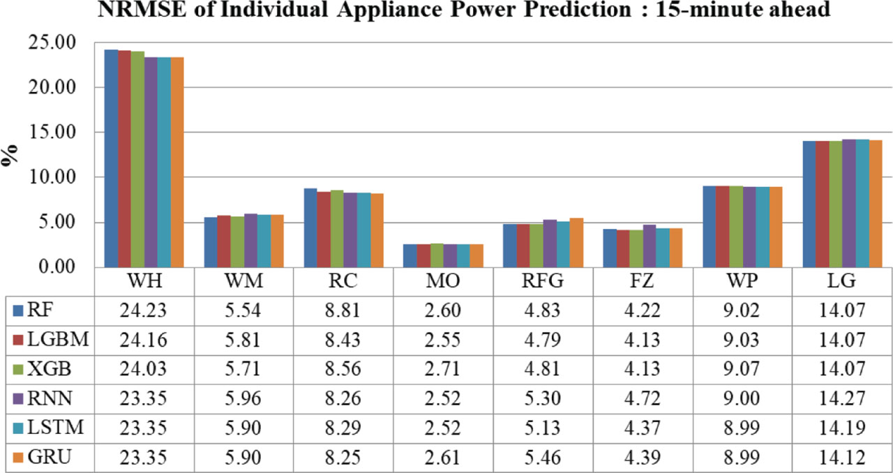
Figure 14:
NRMSE of 15-min ahead prediction. GRU, gated recurrent unit; LGBM, light gradient boosting machine; LSTM, long short-term memory; MO, microwave oven; NRMSE, normalized root mean square error; RF, random forest; RNN, recurrent neural network; WP, Water pump; XGB, extreme gradient boosting; FZ, freezer; LG, lighting; RC, rice cooker; RFG, refrigerator; WH, water heater; WM, washing machine.
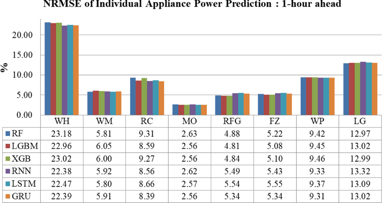
Figure 15:
NRMSE of 1-hr ahead individual appliance power prediction. GRU, gated recurrent unit; LGBM, light gradient boosting machine; LSTM, long short-term memory; MO, microwave oven; NRMSE, normalized root mean square error; RF, random forest; RNN, recurrent neural network; WP, Water pump; XGB, extreme gradient boosting; FZ, freezer; LG, lighting; RC, rice cooker; RFG, refrigerator; WH, water heater; WM, washing machine.
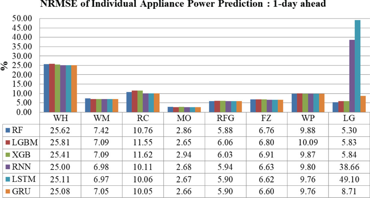
Figure 16:
NRMSE of 1-day ahead individual appliance power prediction. GRU, gated recurrent unit; LGBM, light gradient boosting machine; LSTM, long short-term memory; MO, microwave oven; NRMSE, normalized root mean square error; RF, random forest; RNN, recurrent neural network; WP, Water pump; XGB, extreme gradient boosting; FZ, freezer; LG, lighting; RC, rice cooker; RFG, refrigerator; WH, water heater; WM, washing machine.
Table 4:
NRMSE comparison of individual appliance power prediction
| Time horizon | Lowest NRMSE (%) (appliance, method) | |||
|---|---|---|---|---|
| Reschedulable load | Non-reschedulable load | |||
| Tree-based algorithm | Deep-learning algorithm | Tree-based algorithm | Deep-learning algorithm | |
| 1-min | 2.63 (MO, LGBM) | 2.45 (MO, RNN) | 3.33 (WP, LGBM) | 3.14 (RFG, GRU) |
| 15-min | 2.55 (MO, LGBM) | 2.52 (MO, RNN/LSTM) | 4.13 (FZ, LGBM/XGB) | 4.37 (FZ, LSTM) |
| 1-hr | 2.56 (MO, LGBM/XGB) | 2.56 (MO, GRU) | 4.81 (RFG, LGBM) | 5.34 (RFG/FZ, GRU) |
| 1-day | 2.65 (MO, LGBM) | 2.66 (MO, GRU) | 5.30 (LG, RF) | 5.90 (RFG, LSTM/GRU) |
[i] GRU, gated recurrent unit; LGBM, light gradient boosting machine; LSTM, long short-term memory; MO, microwave oven; NRMSE, normalized root mean square error; RF, random forest; RNN, recurrent neural network; XGB, extreme gradient boosting; FZ, freezer; LG, lighting; RFG, refrigerator; WP, water pump.
For reschedulable load, the MO achieves the lowest NRMSE for all scenarios. At very short-term time horizons (1-min and 15-min), the tree-based model shows slight superiority over the deep learning model. Oppositely, at 1-hr and 1-day time horizons, the deep learning model shows slight superiority over tree-based models.
For non-reschedulable load, no single appliance achieves the lowest NRMSE across all scenarios. The tree-based models outperform deep learning at longer time horizons.
Overall comparison in Table 4 indicates that tree-based models perform better at predicting non-reschedulable loads, while deep learning models perform better for reschedulable loads.
Figures 17 and 18 show the NMAE and NRMSE of multi-horizon average appliance power predictions, respectively. Figure 17 shows that the RF achieves the lowest NMAE of 0.69% for a 1-min time horizon, the RNN achieves the lowest NMAE of 3.06% for a 15-min time horizon, the GRU achieves the lowest NMAE of 2.88% for a 1-hr time horizon, and the RF achieves the lowest NMAE of 3.84% for a 1-day time horizon.
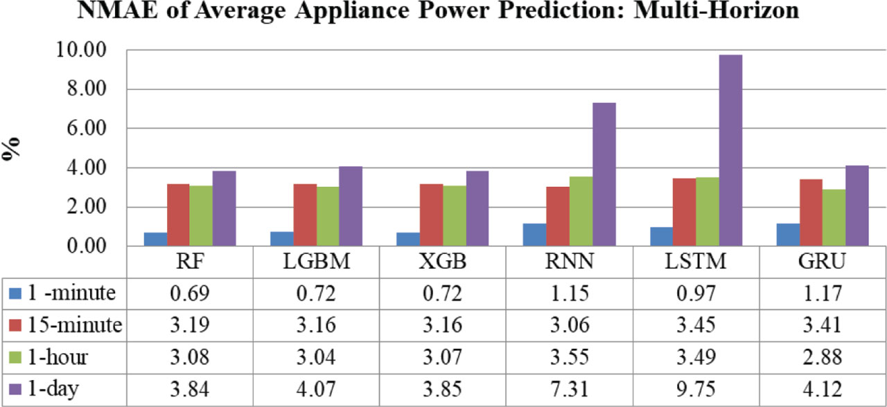
Figure 17:
NMAE of multi-horizon average appliance power prediction. GRU, gated recurrent unit; LGBM, light gradient boosting machine; LSTM, long short-term memory; NMAE, normalized mean absolute error; RF, random forest; RNN, recurrent neural network; XGB, extreme gradient boosting.
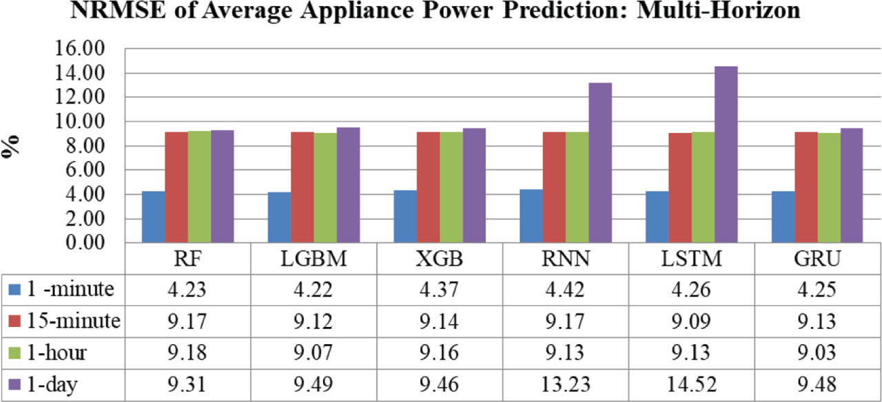
Figure 18:
NRMSE of multi-horizon average appliance power prediction. GRU, gated recurrent unit; LGBM, light gradient boosting machine; LSTM, long short-term memory; NRMSE, normalized root mean square error; RF, random forest; RNN, recurrent neural network; XGB, extreme gradient boosting.
Figure 18 shows that the LGBM achieves the lowest NRMSE of 4.22% for a 1-min time horizon, the LSTM achieves the lowest NRMSE of 9.09% for a 15-min time horizon, the GRU achieves the lowest NRMSE of 9.03% for a 1-hr time horizon, and the RF achieves the lowest NRMSE of 9.31% for a 1-day time horizon. The above results suggest that the tree-based models outperform the deep learning models for multi-horizon average appliance power prediction at the very short (1-min) and long (1-day) time horizons.
Figures 17 and 18 demonstrate that the NMAE and NRMSE increase when the time horizon increases for all prediction techniques. It suggests that prediction accuracy decreases as the forecasting interval increases. Both tree-based and deep-learning models face increasing difficulty in capturing the underlying appliance behavior.
c. Evaluation of total power prediction
Figures 19–22 depict the NMAE of total power predictions for 1-min, 15-min, 1-hr, and 1-day time horizons. In each figure, the NMAEs for six methods are compared across four different feature groups. The comparison results are summarized in Table 5. Table 5 shows that the lowest NMAE of 2.03% is achieved by the Feature Group-C using an LGBM or XGB at a 1-min horizon for the tree-based algorithm, and the lowest NMAE of 2.53% is achieved by the Feature Group-C using GRU at a 1-min horizon for the deep learning algorithm.
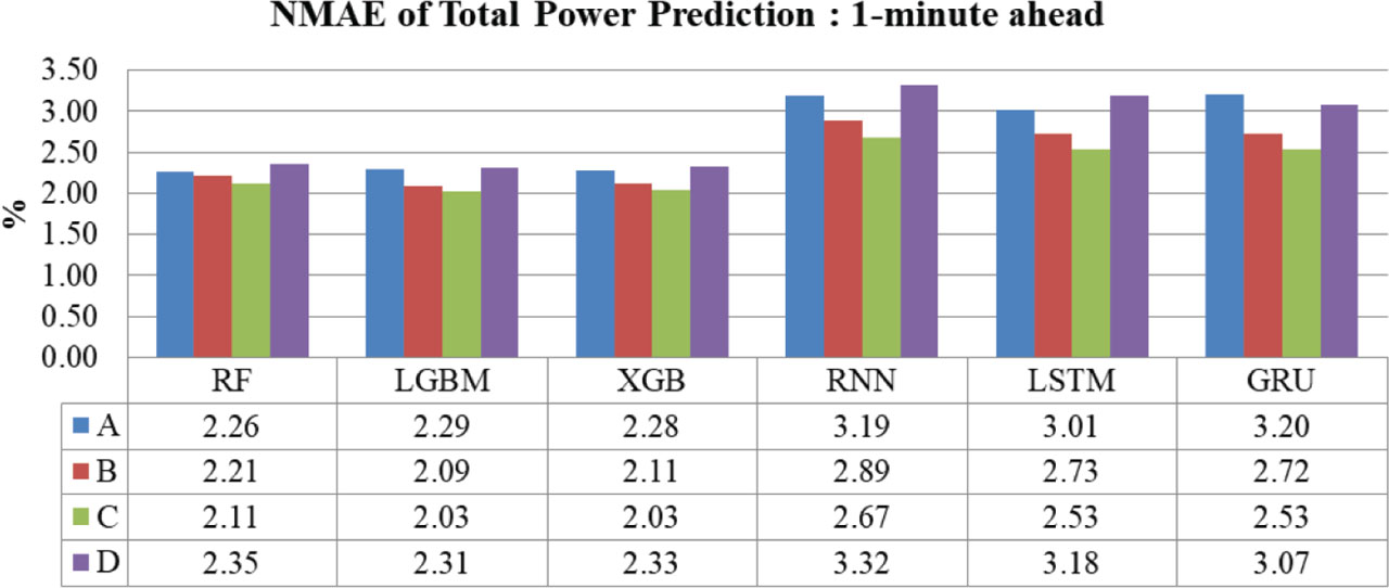
Figure 19:
NMAE of 1-min ahead total power prediction. GRU, gated recurrent unit; LGBM, light gradient boosting machine; LSTM, long short-term memory; NMAE, normalized mean absolute error; RF, random forest; RNN, recurrent neural network; XGB, extreme gradient boosting.
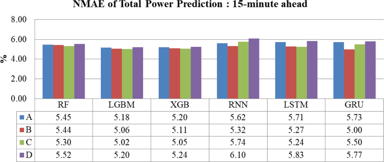
Figure 20:
NMAE of 15-min ahead total power prediction. GRU, gated recurrent unit; LGBM, light gradient boosting machine; LSTM, long short-term memory; NMAE, normalized mean absolute error; RF, random forest; RNN, recurrent neural network; XGB, extreme gradient boosting.
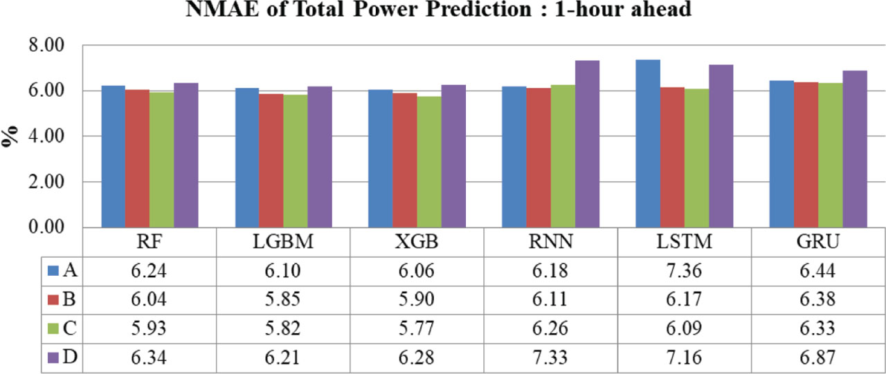
Figure 21:
NMAE of 1-hr ahead total power prediction. GRU, gated recurrent unit; LGBM, light gradient boosting machine; LSTM, long short-term memory; NMAE, normalized mean absolute error; RF, random forest; RNN, recurrent neural network; XGB, extreme gradient boosting.
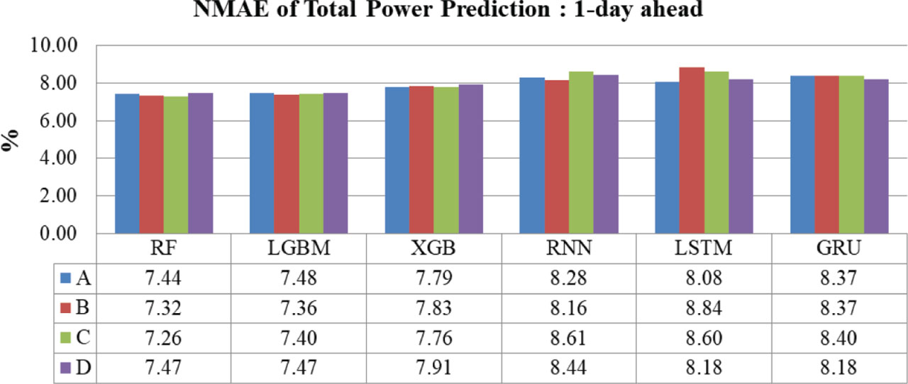
Figure 22:
NMAE of 1-day ahead total power prediction. GRU, gated recurrent unit; LGBM, light gradient boosting machine; LSTM, long short-term memory; NMAE, normalized mean absolute error; RF, random forest; RNN, recurrent neural network; XGB, extreme gradient boosting.
Table 5:
NMAE comparison of total power prediction
| Time horizon | Lowest NMAE (%) (feature, method) | |
|---|---|---|
| Tree-based algorithm | Deep learning algorithm | |
| 1-min | 2.03 (C, LGBM/XGB) | 2.53 (C, LSTM/GRU) |
| 15-min | 5.02 (C, LGBM) | 5.00 (B, GRU) |
| 1-hr | 5.77 (C, XGB) | 6.09 (C, LSTM) |
| 1-day | 7.26 (C, RF) | 8.08 (A, LSTM) |
For the tree-based algorithm, Feature Group-C achieves the lowest NMAE across all time horizons, where LGBM is superior at 1-min and 15-min time horizons, XGB is superior at 1-min and 1-hr, and RF is superior at 1-day. It suggests that the Feature Group-C, which combines all appliance power consumption and total power as the input features of the prediction models, effectively reduces the NMAE.
For the deep learning algorithm, Feature Group-C achieves the lowest NMAE at 1-min and 1-hr time horizons, where GRU is superior, and LSTM is superior at 1-hr and 1-day time horizons. Feature Group-A achieves the lowest NMAE at 1-day time horizon using the LSTM. Again, the Feature Group-C effectively reduces the NMAE, especially for very short-term prediction.
Figures 23–26 depict the NRMSE of total power predictions for 1-min, 15-min, 1-hr, and 1-day time horizons. In each figure, the NRMSEs for six methods are compared across four different feature groups. The comparison results are summarized in Table 6, where the lowest NRMSE of 4.61% is achieved by the Feature Group-C using an LGBM at a 1-min horizon for the tree-based algorithm, and the lowest NRMSE of 4.91% is achieved by the Feature Group-C using GRU at a 1-min horizon for the deep learning algorithm.
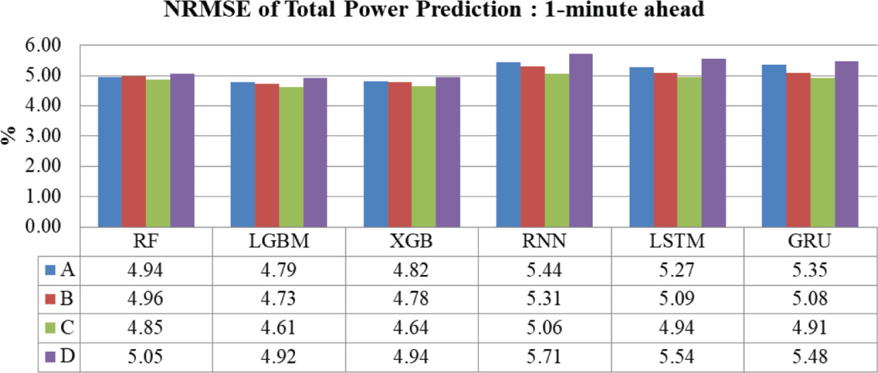
Figure 23:
NRMSE of 1-min ahead total power prediction. GRU, gated recurrent unit; LGBM, light gradient boosting machine; LSTM, long short-term memory; NRMSE, normalized root mean square error; RF, random forest; RNN, recurrent neural network; XGB, extreme gradient boosting.
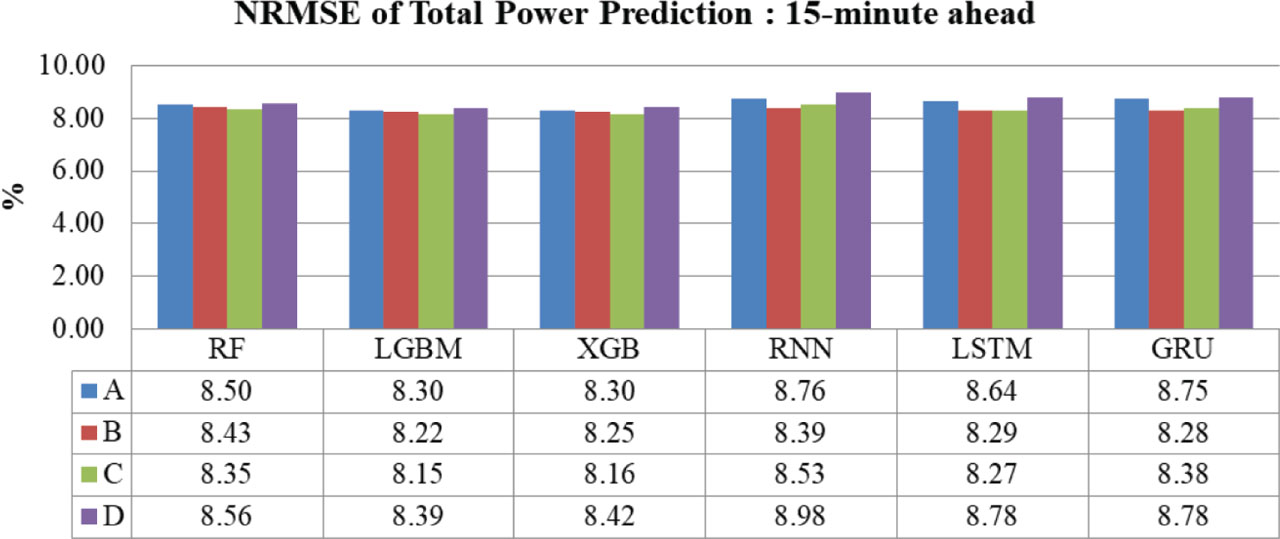
Figure 24:
NRMSE of 15-min ahead total power prediction. GRU, gated recurrent unit; LGBM, light gradient boosting machine; LSTM, long short-term memory; NRMSE, normalized root mean square error; RF, random forest; RNN, recurrent neural network; XGB, extreme gradient boosting.
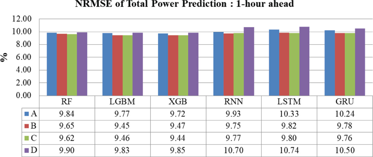
Figure 25:
NRMSE of 1-hr ahead total power prediction. GRU, gated recurrent unit; LGBM, light gradient boosting machine; LSTM, long short-term memory; NRMSE, normalized root mean square error; RF, random forest; RNN, recurrent neural network; XGB, extreme gradient boosting.
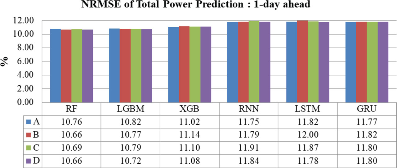
Figure 26:
NRMSE of 1-day ahead total power prediction. GRU, gated recurrent unit; LGBM, light gradient boosting machine; LSTM, long short-term memory; NRMSE, normalized root mean square error; RF, random forest; RNN, recurrent neural network; XGB, extreme gradient boosting.
Table 6:
NRMSE comparison of total power prediction
| Time horizon | Lowest NRMSE (%) (feature, method) | |
|---|---|---|
| Tree-based algorithm | Deep-learning algorithm | |
| 1-min | 4.61 (C, LGBM) | 4.91 (C, GRU) |
| 15-min | 8.15 (C, LGBM) | 8.27 (C, LSTM) |
| 1-hr | 9.44 (C, XGB) | 9.75 (B, RNN) |
| 1-day | 10.66 (B/D, RF) | 11.75 (A, RNN) |
For the tree-based algorithm, Feature Group-C achieves the lowest NRMSE at very short-term time horizons, where LGBM is superior at 1-min and 15-min time horizons, XGB is superior at 1-hr. Feature Group B and D achieve the lowest NRMSE at 1-day using the RF. It suggests that the Feature Group-C effectively reduces the NRMSE, especially for very short-term prediction.
For the deep learning algorithm, Feature Group-C achieves the lowest NRMSE at very short-term time horizons, where GRU is superior at a 1-min time horizon, LSTM at a 15-min time horizon. Feature Group-B achieves the lowest NRMSE at 1-hr time horizon using the RNN. Feature Group-A achieves the lowest NRMSE at 1-day using the RNN. Similarly, before that, the Feature Group-C effectively reduces the NRMSE, especially for very short-term prediction.
Figures 27 and 28 show the NMAE and NRMSE of multi-horizon total power predictions, respectively. Figure 27 shows that the Feature Group-C achieves the lowest NMAE of 2.32% for a 1-min time horizon, the Feature Group-B achieves the lowest NMAE of 5.20% for a 15-min time horizon, the Feature Group-C achieves the lowest NMAE of 6.03% for a 1-hr time horizon, and the Feature Group-A achieves the lowest NMAE of 7.91% for a 1-day time horizon.
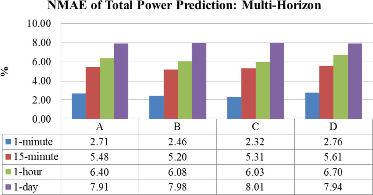
Figure 27:
NMAE of multi-horizon total power prediction. NMAE, normalized mean absolute error.
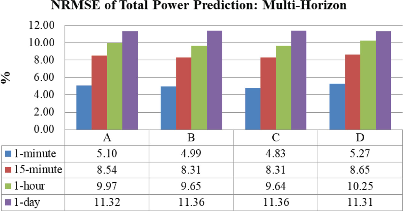
Figure 28:
NRMSE of multi-horizon total power prediction. NRMSE, normalized root mean square error.
Figure 28 shows that Feature Group-C achieves the lowest NRMSE of 4.83% for a 1-min time horizon, the lowest NRMSE of 8.31% for a 15-min time horizon, the lowest NRMSE of 9.64% for a 1-hr time horizon, and Feature Group-D achieves the lowest NRMSE of 11.31% for a 1-day time horizon. The results suggest that the Feature Group-C is an effective feature in multi-horizon average total power prediction, especially for the very short-term forecasting.
Figures 27 and 28 demonstrate that the NMAE and NRMSE increase when the time horizon increases, regardless of feature group. A longer horizon makes it harder for the algorithm to capture the model, even with several features adopted.
d. Evaluation summary
From previous discussions, several findings can be summarized as follows:
Individual appliance power prediction:
The NMAE comparison shows that deep learning models are advantageous for short-term forecasting and appliances with complex temporal behavior. In contrast, tree-based models are more effective for longer horizons or appliances with stable usage patterns.
The NRMSE comparisons show that tree-based models are more effective for non-reschedulable loads, while deep-learning models provide advantages for forecasting of reschedulable loads.
The NMAE and NRMSE increase with the time horizon, regardless of the prediction algorithm. It indicates that the prediction algorithm becomes increasingly challenging to capture the underlying appliance behavior over a longer horizon.
Total power prediction:
Feature Group-C, which combines all individual appliance power consumption with total power, achieves the lowest NMAE and NRMSE across most horizons for both tree-based and deep-learning models, particularly for very short-term forecasts.
Among tree-based methods, no single model performs across multiple horizons. In deep learning, GRUs and LSTMs dominate short-term horizons.
The NMAE and NRMSE increase when the time horizon increases, regardless of feature group. It indicates that the algorithm is more complicated to capture the model, even with several features adopted.
The appliance-specific, horizon-dependent model selection strategy is essential for optimizing prediction accuracy in HEMS.
Incorporating all individual appliance power measurements, along with total power, as model inputs enhances total power prediction accuracy.
IV. Conclusion
This paper presented a comprehensive multi-horizon prediction framework for home energy consumption that simultaneously considers individual appliance loads and total household power. An IoT-based SCADA monitoring system was used to collect the home appliance power consumption. The approach was evaluated using six machine learning techniques, comprising tree-based and deep learning models, across four forecasting horizons. The evaluation results for NMAE and NRMSE show that deep learning techniques are more effective for short-term predicting the individual appliance power. Meanwhile, tree-based algorithms are superior for longer prediction horizons and for appliances with stable usage patterns. The most valuable finding is that combining appliance-level power measurements significantly improves the accuracy of total power prediction.
Future work may extend this research by integrating weather data, user behavior patterns, and occupancy information, and by exploring advanced algorithms to enhance predictive capability further.
Acknowledgment
The authors thank the Institute for Research and Community Service ITN Malang for funding this research. (Research funding No.: ITN.07.037.011/I. LPPM/2025).