
Table 1:
Insights from the literature review on deep learning approaches for emotion and stress detection
| No. | Author name and year | Methodology used | Limitations |
|---|---|---|---|
| 1 | Seo et al. (2022) [9] | Multimodal deep neural network | Declined performance in multilevel classification; dependence on sensors limits scalability |
| 2 | Campanella et al. (2023) [10] | Random forest, SVM, logistic regression | Handcrafted features; limited subject diversity affects generalizability |
| 3 | Li & Lima (2021) [11] | ResNet-50 | Poor robustness in real-world settings; limited generalization |
| 4 | Gupta et al. (2023) [12] | Inception-V3, VGG19, ResNet-50 | Ignores contextual/behavioral cues; focuses solely on facial expressions |
| 5 | Mohan et al. (2021) [13] | FER-net | Inconsistent performance across datasets; generalization remains a challenge |
| 6 | Khattak et al. (2022) [14] | CNN | Relies on static facial images, limiting its ability to capture temporal variations essential for video-based emotion analysis |
| 7 | Savchenko et al. (2022) [15] | Fine-tuned CNN | Limited to static image models; lacks dynamic emotion tracking |
| 8 | Minaee et al. (2021) [16] | Deep-emotion (attentional CNN) | No temporal modeling; dependent on labeled datasets for accuracy |
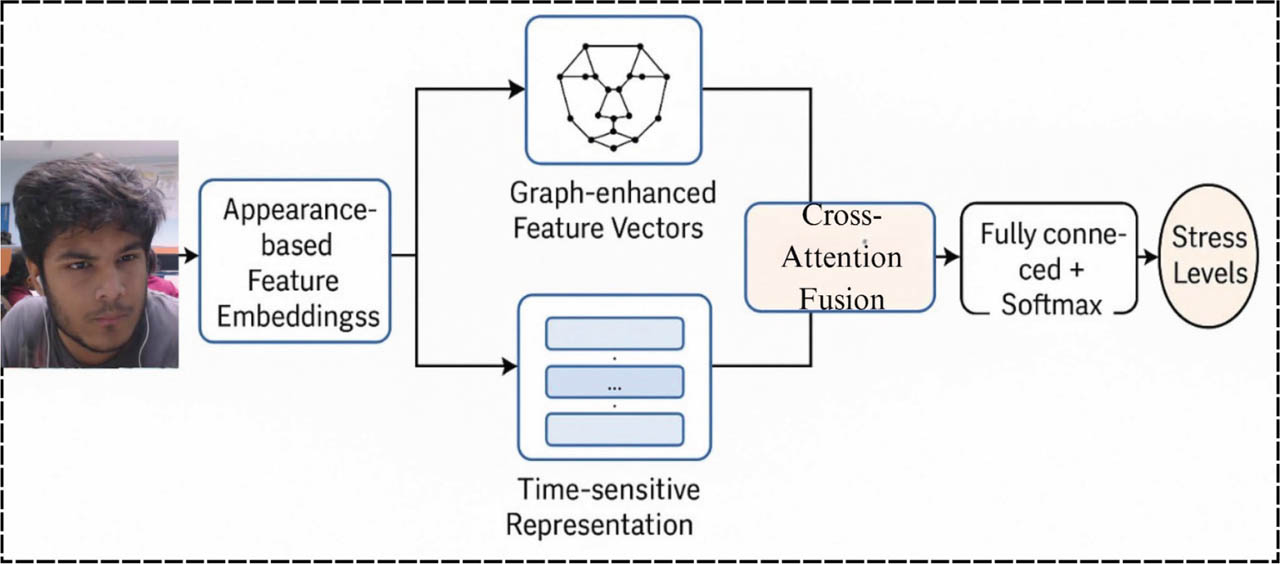
Figure 1:
Architecture diagram of the proposed model.
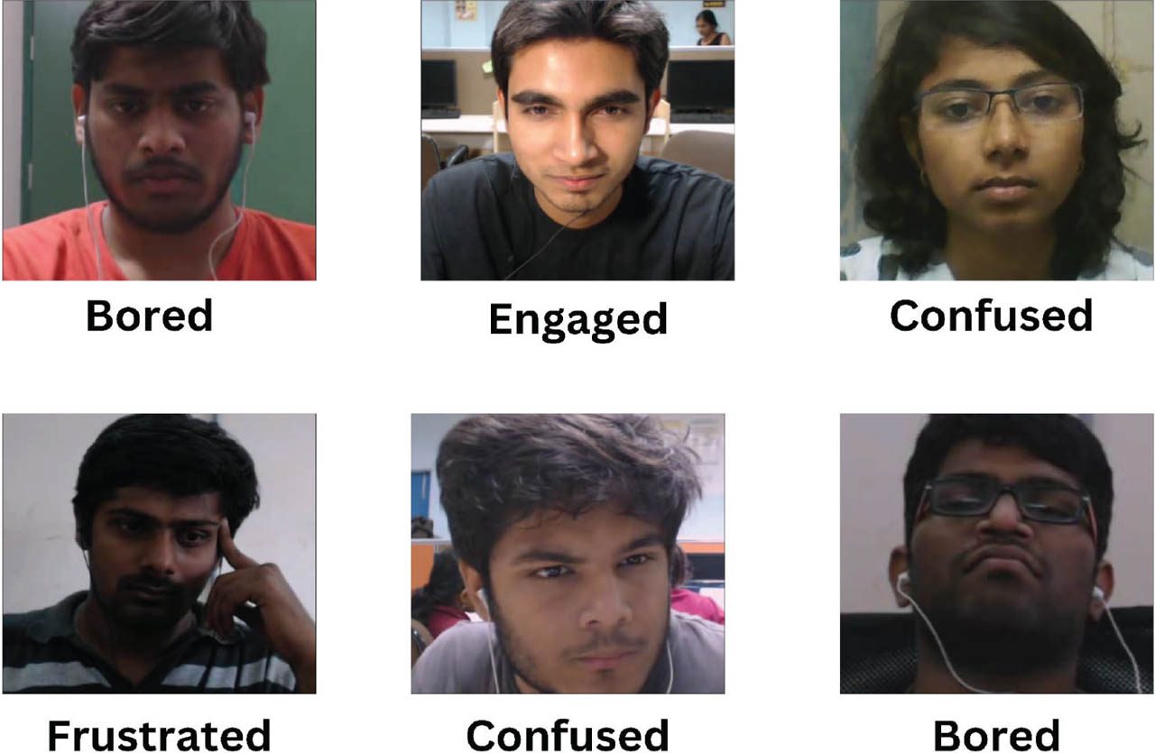
Figure 2:
Sample images from the DAiSEE dataset representing affective states. DAiSEE, dataset for affective states in e-environments.
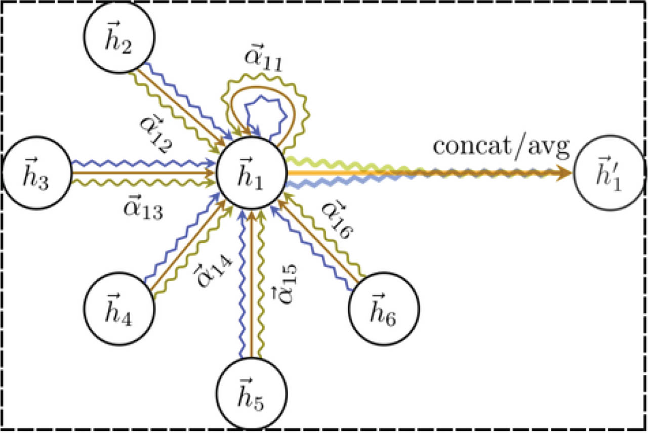
Figure 3:
Architecture diagram of the GAT. GAT, graph attention network.
Table 2:
Sample output feature vectors from GAT for five facial landmark nodes
| Node ID | Feature 1 | Feature 2 | Feature 3 | Feature 4 |
|---|---|---|---|---|
| Node 1 (left eye corner) | 0.348 | 0.621 | 0.214 | 0.489 |
| Node 2 (right eye corner) | 0.457 | 0.582 | 0.199 | 0.501 |
| Node 3 (nose tip) | 0.511 | 0.403 | 0.255 | 0.620 |
| Node 4 (left mouth corner) | 0.398 | 0.634 | 0.201 | 0.537 |
| Node 5 (right mouth corner) | 0.442 | 0.593 | 0.228 | 0.511 |
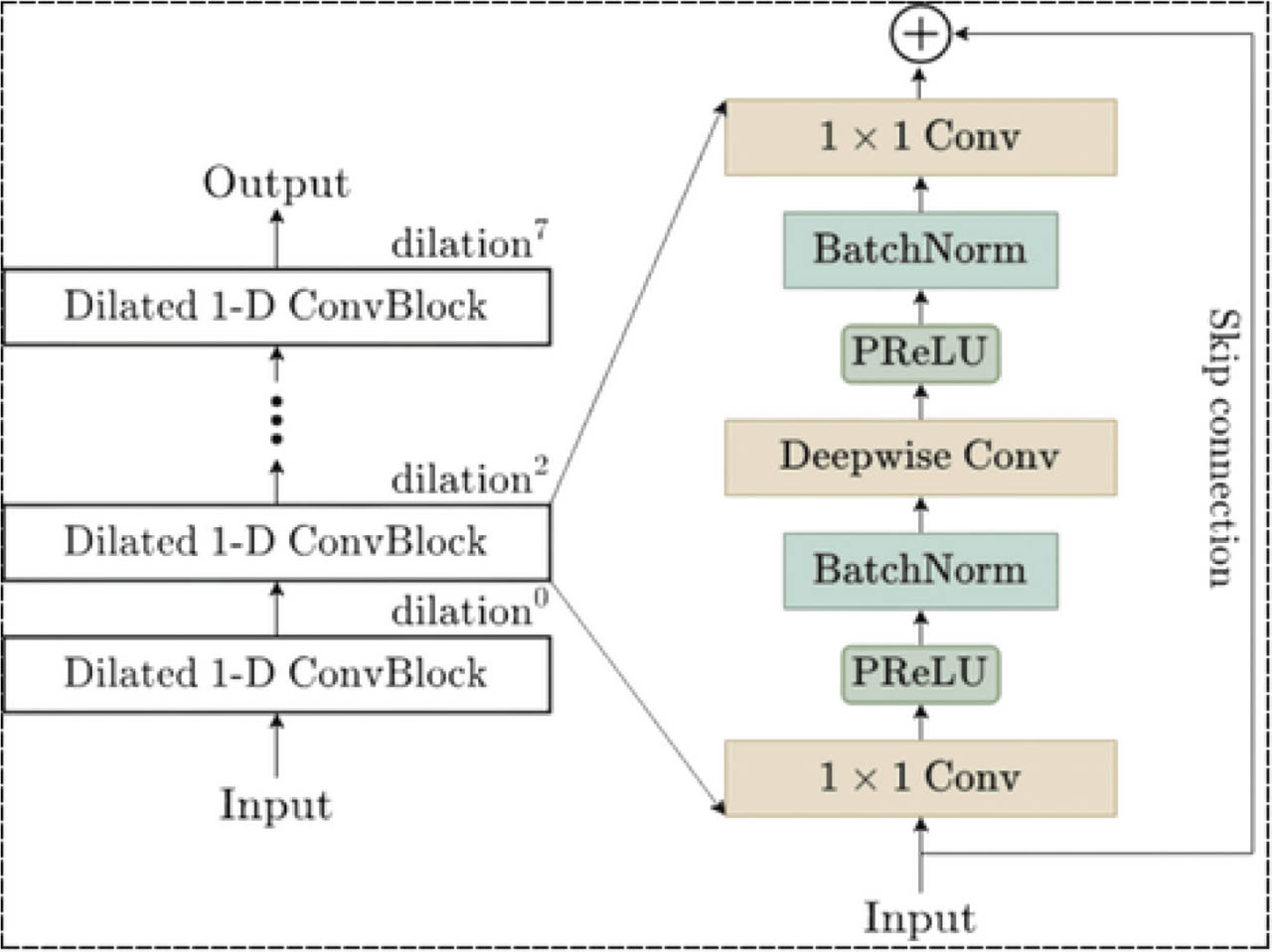
Figure 4:
Architecture diagram of the TCN. TCN, temporal convolutional network.
Table 3:
TCN-generated temporal feature vector (for a sequence of five frames)
| Time step (t) | Feature 1 | Feature 2 | Feature 3 | Feature 4 |
|---|---|---|---|---|
| Frame 1 | 0.421 | 0.359 | 0.288 | 0.612 |
| Frame 2 | 0.437 | 0.370 | 0.295 | 0.601 |
| Frame 3 | 0.458 | 0.390 | 0.302 | 0.593 |
| Frame 4 | 0.469 | 0.408 | 0.310 | 0.585 |
| Frame 5 | 0.482 | 0.427 | 0.320 | 0.578 |
Table 4:
Spatiotemporal feature embedding (after STG-TCN fusion)
| Frame No. | Attention-weighted feature 1 | Feature 2 | Feature 3 | ... | Feature 128 |
|---|---|---|---|---|---|
| Frame 1 | 0.045 | 0.082 | −0.017 | ... | 0.103 |
| Frame 2 | 0.051 | 0.091 | −0.009 | ... | 0.110 |
| Frame 3 | 0.063 | 0.104 | 0.002 | ... | 0.123 |
| Frame 4 | 0.059 | 0.099 | −0.001 | ... | 0.118 |
| Frame 5 | 0.066 | 0.107 | 0.005 | ... | 0.127 |
| Input: Video V with T frames |
| 1. Preprocessing and Landmark Extraction: for each frame F_t in video V do |
| face ← MTCNN (F_t) |
| landmarks _t ← Dlib68 (face) |
| end for |
| 2. Spatial Feature Extraction using GAT: |
| Construct graph G(V, E) from _ landmarks _t → nodes = landmarks, edges = anatomical connectivity |
| for each graph G _t do |
| spatial _feat _t ← GAT (G _t) |
| end for |
| 3. Temporal Feature Extraction using TCN: for each frame F _t in video V do |
| embedding _t ← EfficientNet_Lite(F_t) |
| end for |
| temporal _feat ← TCN({embedding_1, ..., embedding_T}) |
| 4. Cross-Attention Fusion: for each time step t do |
| attention _ weights ← CrossAttention(spatial_feat_t, temporal_feat_t) |
| fused _feat _t ← attention _ weights spatial⊗ |
| [spatial _ feat _ t || temporal _ feat _ t] |
| end for |
| 5. Spatio-Temporal Feature Aggregation: |
| unified _representation ← Aggregate({fused_feat_1, ..., fused_feat_T}) |
| 6. Classification: |
| logits ← FullyConnected(unified_representation) |
| stress _level ← Softmax(logits) |
| Return: stress _level |
| Output: Predicted stress level {Low, Medium, High} |
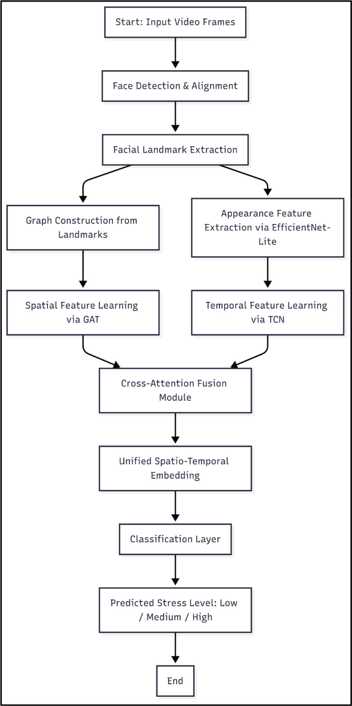
Figure 5:
Flowchart for the proposed model. GAT, graft attention network; TCN, temporal convolutional networks.
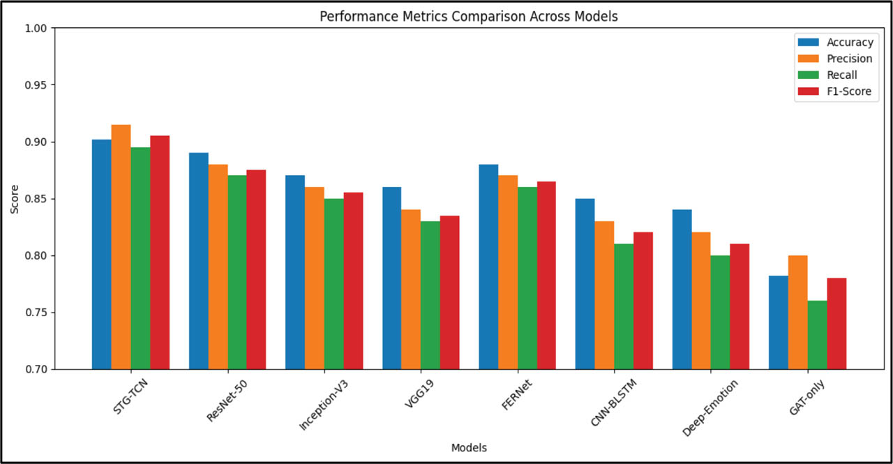
Figure 6:
Comprehensive performance metrics comparison of STG-TCN versus baseline models.
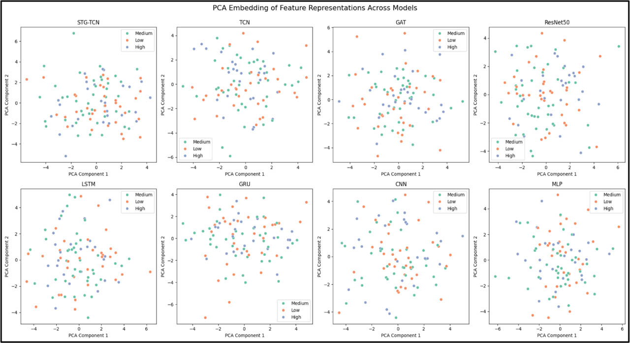
Figure 7:
PCA embedding of feature representations across models. GAT, graft attention network; PCA, principal component analysis; TCN, temporal convolutional networks.
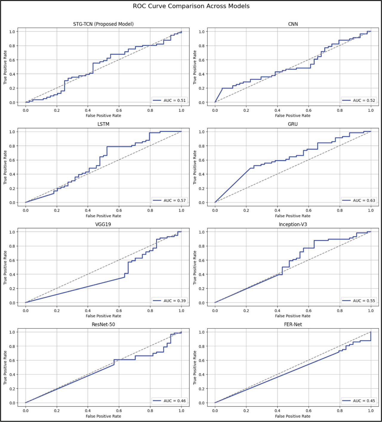
Figure 8:
ROC curve comparison across models.
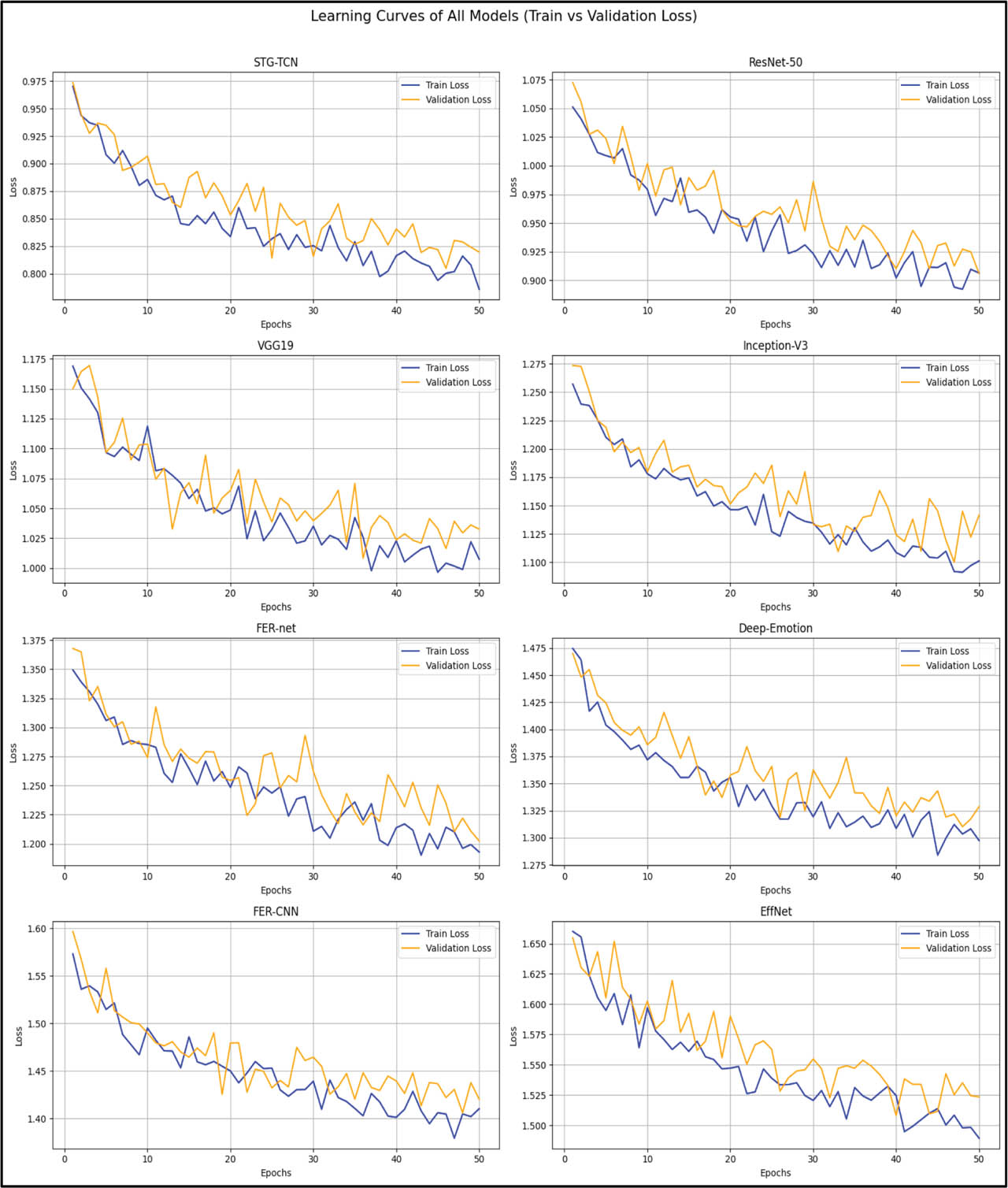
Figure 9:
Learning curves of train and validation loss for various models.
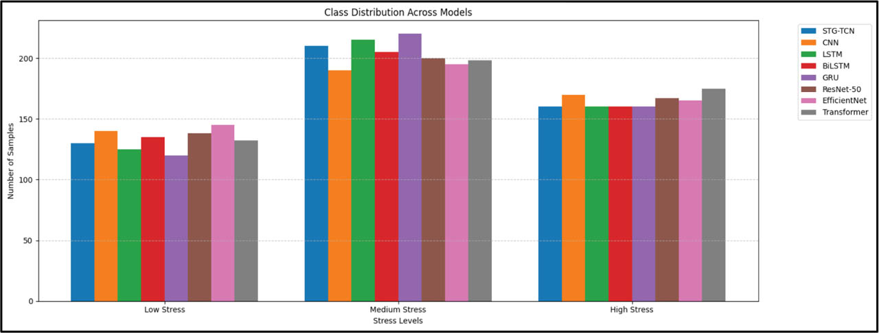
Figure 10:
Class distribution across various compared models.