
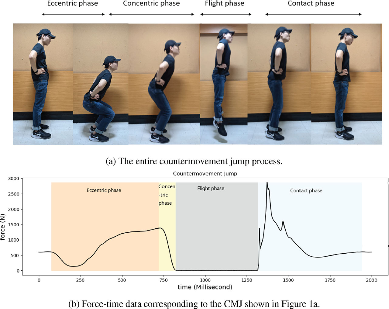
Figure 1:
The process and corresponding force-time data of a CMJ. (A) The entire CMJ process. (B) Force-time data corresponding to the CMJ shown in (A). CMJ, countermovement jump.
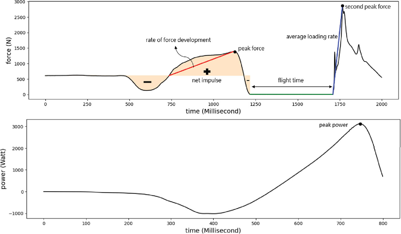
Figure 2:
Seven performance variables used to assess CMJ, derived from the force-time curve and the power-time curve. CMJ, countermovement jump.
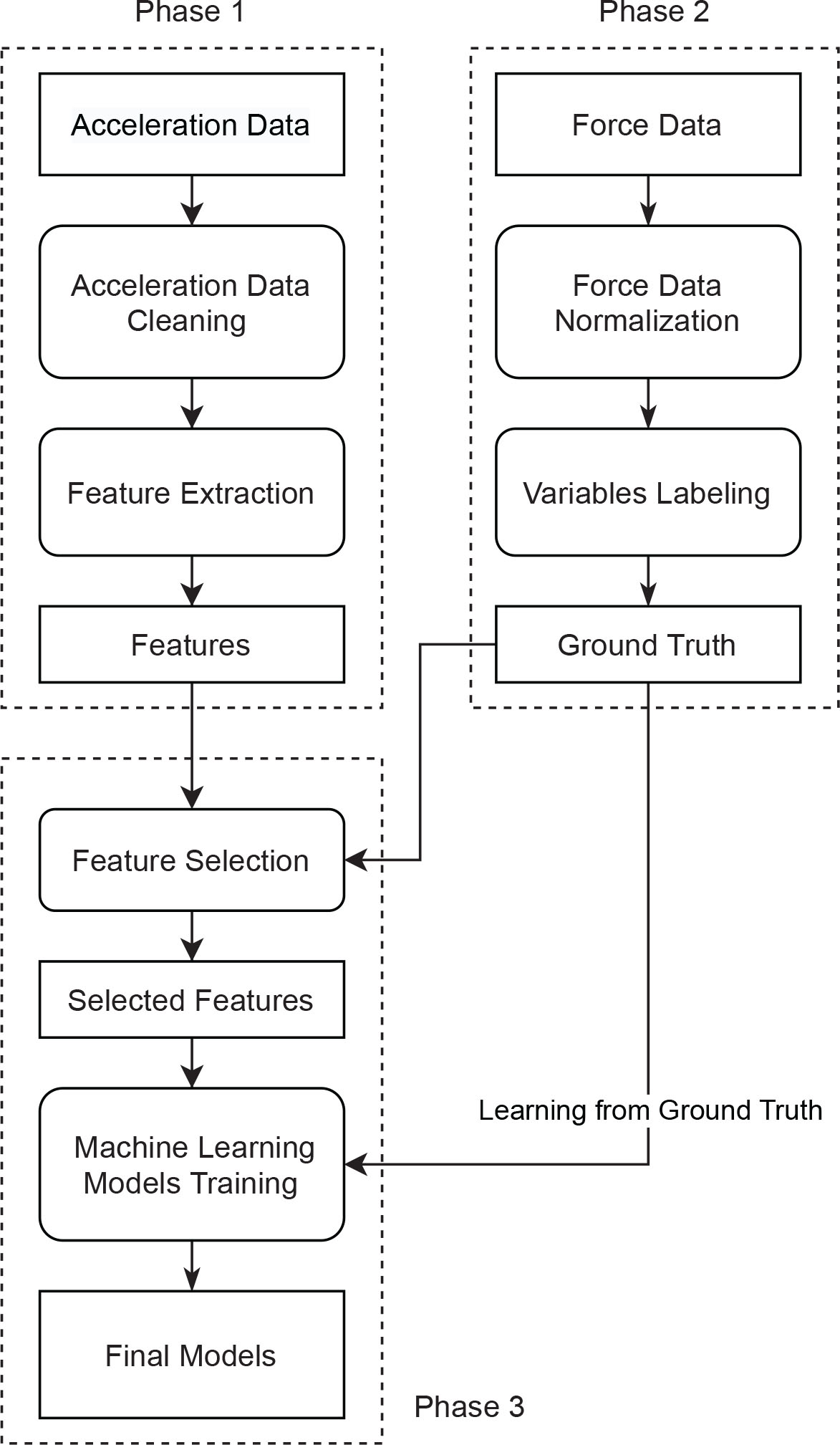
Figure 3:
Proposed architecture and application workflow for a machine learning model that can predict CMJ performance variables from IMU sensor data. CMJ, countermovement jump; IMU, inertial measurement unit.
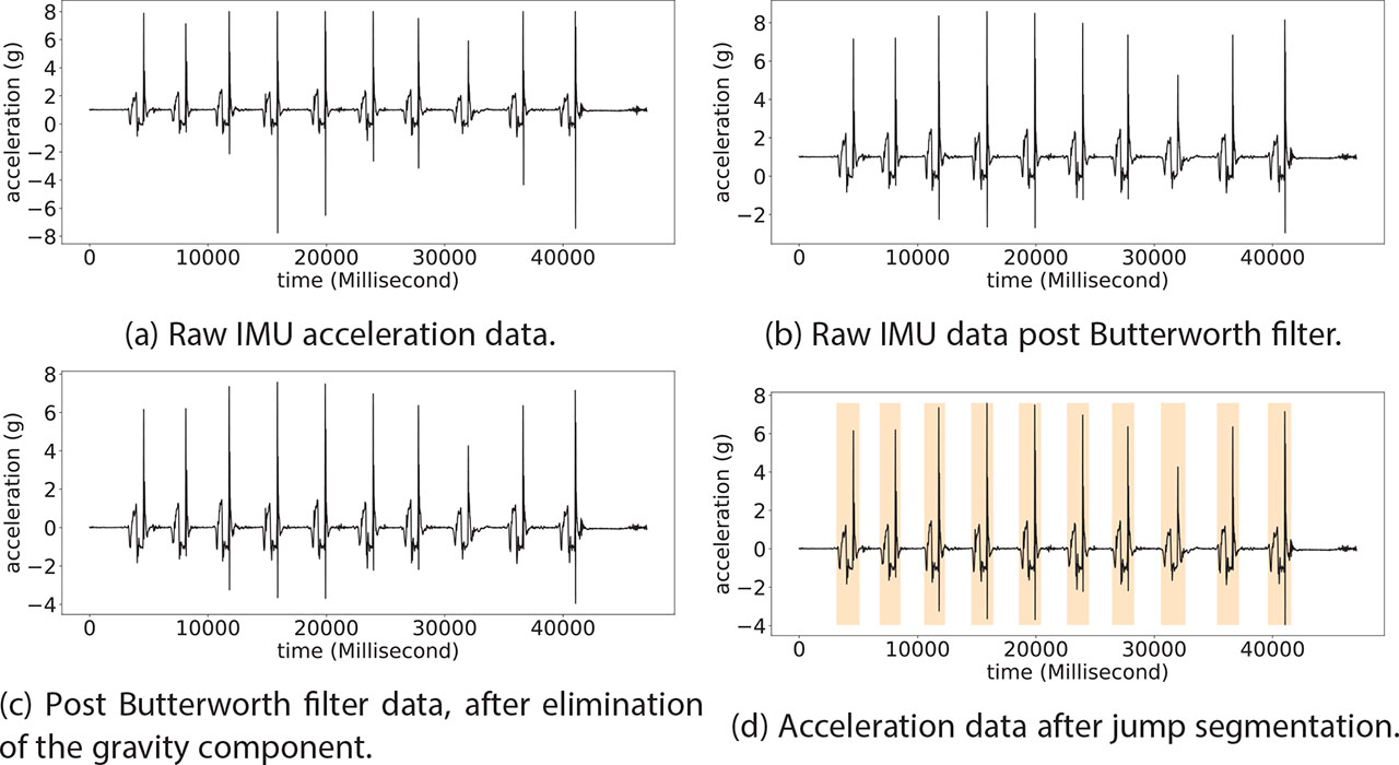
Figure 4:
Data preprocessing of CMJ acceleration data. (A) Raw IMU acceleration data (B) Raw IMU data post-Butterworth filter. (C) Post-Butterworth filter data, after elimination of the gravity component. (D) Acceleration data after jump segmentation. CMJ, countermovement jump; IMU, inertial measurement unit.
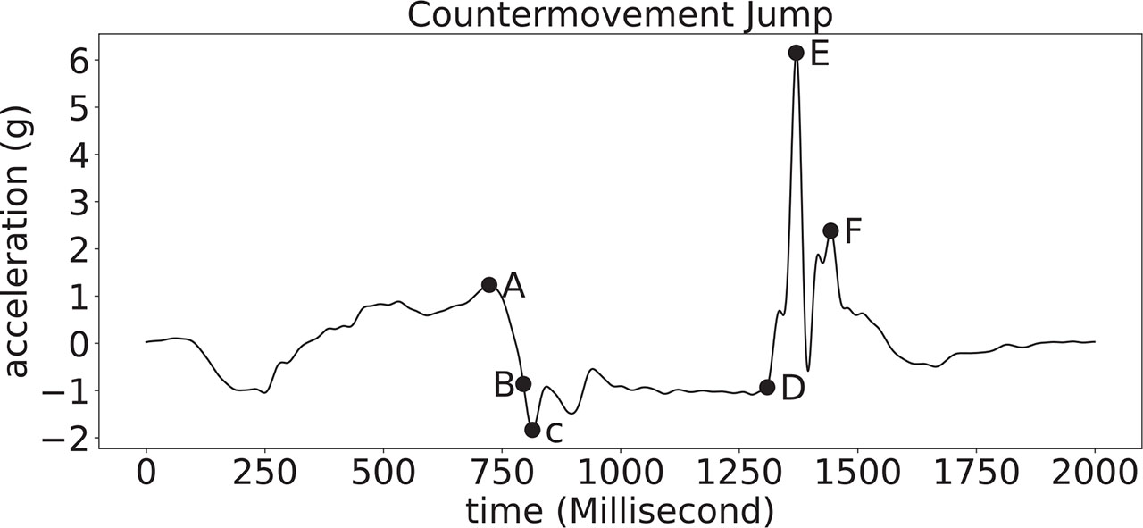
Figure 5:
Critical point extraction from post-processed IMU acceleration-time data. IMU, inertial measurement unit.
Table 1:
31 features extracted from the acceleration data
| Feature | Description |
|---|---|
| Mean | The mean of the acceleration data |
| SD | The standard deviation of the acceleration data |
| IQR | The interquartile range of the acceleration data |
| Skewness | The skewness of the acceleration data |
| Kurtosis | The kurtosis of the acceleration data |
| Frequency | The dominant frequency of the acceleration data |
| Entropy | The sample entropy of the acceleration data |
| value_A | The value of point A |
| value_C | The value of point C |
| value_E | The value of point E |
| value_F | The value of point F |
| duration_AC | The time interval from point A to point C |
| duration_BD | The time interval from point B to point D |
| duration_CE | The time interval from point C to point E |
| duration_EF | The time interval from point E to point F |
| slope_AL | The slope from (point A − 20 ms) to point A |
| slope_AR | The slope from point A to (point A + 20 ms) |
| slope_CL | The slope from (point C − 20 ms) to point C |
| slope_CR | The slope from point C to (point C + 20 ms) |
| slope_EL | The slope from (point E − 10 ms) to point E. |
| slope_ER | The slope from point E to (point E + 10 ms). |
| slope_FL | The slope from (point F − 10 ms) to point F |
| slope_FR | The slope from point F to (point F + 10 ms) |
| slope_AC | The slope from point A to point C |
| slope_CE | The slope from point C to point E |
| slope_DE | The slope from point D to point E |
| slope_EF | The slope from point E to point F. |
| Integration | The integration value before point C |
| average_A | The average value between (point A − 80 ms) and (point A + 20 ms) |
| average_C | The average value between (point C − 20 ms) and (point C + 180 ms). |
| average_E | The average value between (point E − 20 ms) and (point E + 180 ms) |
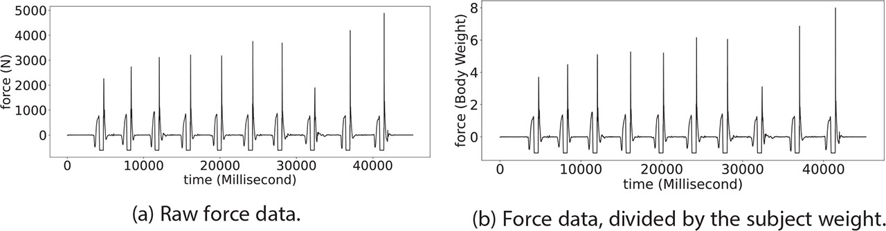
Figure 6:
Data preprocessing of CMJ force data. (A) Raw force data. (B) Force data, divided by the subject weight. CMJ, countermovement jump.

Figure 7:
Data preprocessing of CMJ power data. (A) Raw power data. (B) Power data, divided by the subject weight. CMJ, countermovement jump.
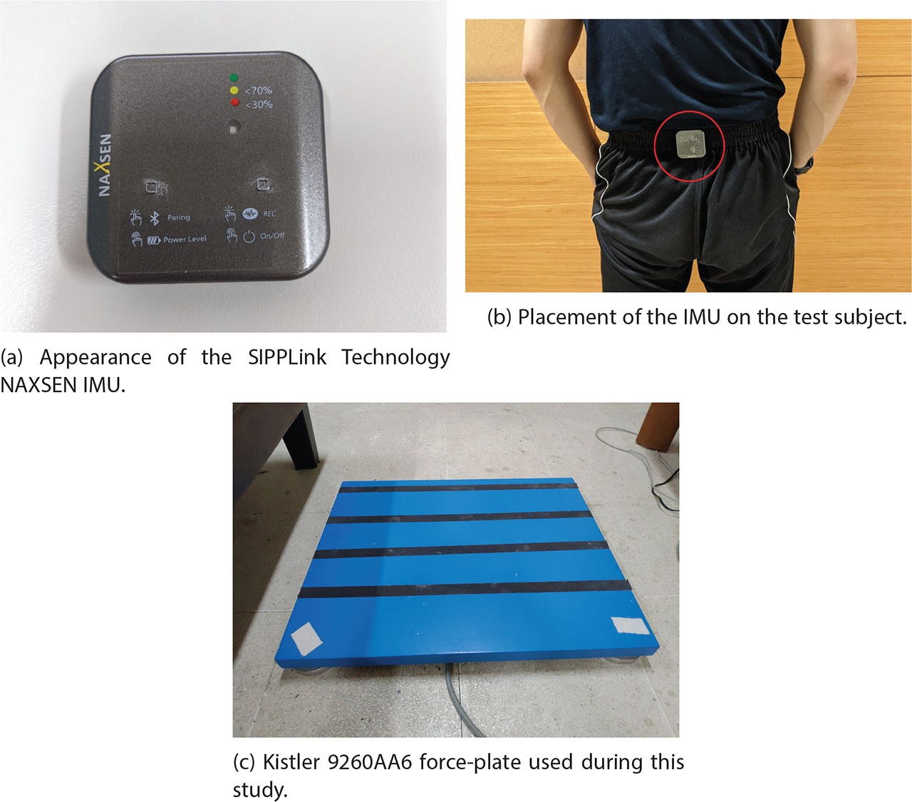
Figure 8:
A NAXSEN IMU tied on a jumper and a Kistler 9260AA6 force plate. (A) Appearance of the SIPPLink Technology. (B) Placement of the IMU on the test subject. (C) Kistler 9260AA6 force plate used during this study. IMU, inertial measurement unit.
Table 2:
Machine learning parameter settings for the models used in this study
| Model | Parameter | Setting value |
|---|---|---|
| LSVR [11] | Epsilon | 0.0 |
| Tol | 0.0001 | |
| C | 1.0 | |
| Loss | epsilon_insensitive | |
| DTR [11] | intercept_scaling | 1.0 |
| max_iter | 100,000 | |
| max_depth | None | |
| min_samples_split | 2 | |
| min_samples_leaf | 1 | |
| min_weight_fraction_leaf | 0.0 | |
| XGBR | max_leaf_nodes | None |
| min_impurity_decrease | 0.0 | |
| learnig_rate | 0.3 | |
| Subsample | 1 | |
| n_estimators | 100 | |
| Gamma | 0.0 | |
| max_depth | 6 | |
| min_child_weight | 1 | |
| max_delta_step | 0 | |
| num_leaves | 31 | |
| max_depth | −1 (no limit) | |
| Subsample | 1 | |
| LGBMR | learning_rate | 0.1 |
| n_estimators | 100 | |
| min_split_gain | 0.0 | |
| min_child_weight | 0.001 | |
| min_child_samples | 20 |
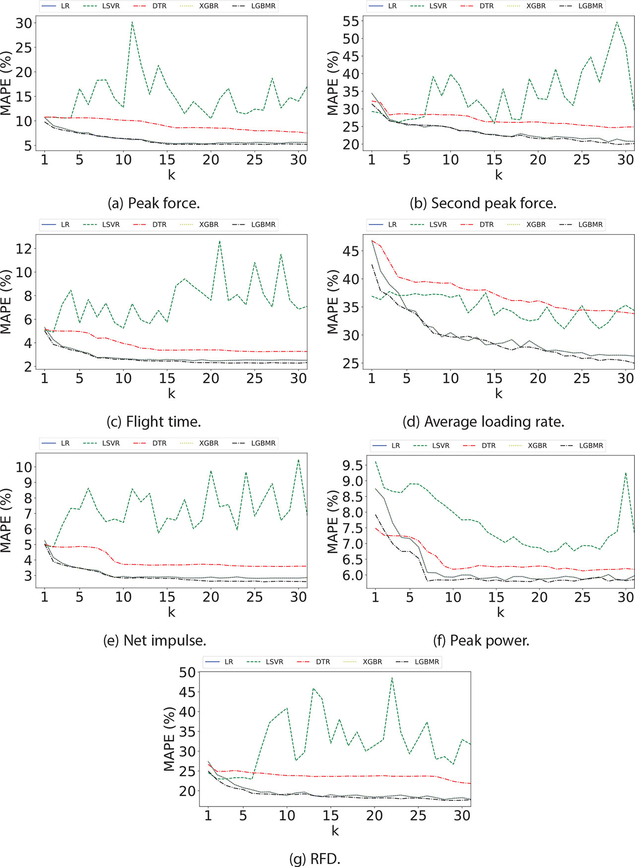
Figure 9:
Prediction results from varying the number (k) of selected features for each performance variable, under each of the five regression models. (A) Peak force. (B) Second peak force. (C) Flight time. (D) Average loading rate. (E) Net impulse. (F). Peak power. (G) RFD. DTR, decision tree regression; LGBMR, light gradient boosting machine regression; LR, linear regression; LSVR, linear support vector regression; MAPE, mean absolute percentage error; RFD, rate of force development; XGBR, eXtreme gradient boosting regression.
Table 3:
Comparison of MAPE for original data and up-sampling data.
| (a) MAPE of different models utilizing the original data (1,000 Hz native). | ||||||
|---|---|---|---|---|---|---|
| Variable | Model | LR [11] | LSVR [11] | DTR [11] | XGBR | LGBMR |
| Peak force | 7.97 | 10.84 | 7.54 | 5.50 | 5.00 | |
| Second peak force | 24.88 | 28.31 | 23.84 | 19.16 | 18.07 | |
| Flight time | 2.59 | 4.63 | 2.85 | 2.09 | 2.04 | |
| Average loading rate | 34.32 | 33.54 | 30.68 | 23.50 | 23.59 | |
| Net impulse | 2.99 | 4.63 | 3.28 | 2.61 | 2.42 | |
| Peak power | 5.73 | 6.86 | 7.21 | 5.60 | 5.43 | |
| RFD | 21.12 | 23.16 | 21.73 | 17.50 | 16.56 | |
| (b) MAPE of different models utilizing up-sampled data (50–1,000 Hz, by duplication). | ||||||
|---|---|---|---|---|---|---|
| Variable | Model | LR [11] | LSVR [11] | DTR [11] | XGBR | LGBMR |
| Peak force | 8.06 | 11.18 | 7.60 | 5.63 | 5.29 | |
| Second peak force | 25.84 | 26.52 | 28.20 | 20.96 | 20.04 | |
| Flight time | 3.52 | 4.87 | 3.22 | 2.52 | 2.38 | |
| Average loading rate | 34.82 | 33.08 | 36.44 | 26.89 | 26.37 | |
| Net impulse | 3.82 | 4.83 | 3.82 | 2.89 | 2.76 | |
| Peak power | 6.36 | 7.28 | 7.84 | 6.11 | 5.91 | |
| RFD | 22.02 | 23.22 | 23.65 | 17.85 | 17.55 | |
| (c) MAPE of different models utilizing up-sampled data (50–1,000 Hz, by interpolation) | ||||||
|---|---|---|---|---|---|---|
| Variable | Model | LR [11] | LSVR [11] | DTR [11] | XGBR | LGBMR |
| Peak force | 7.50 | 10.27 | 7.32 | 5.59 | 5.18 | |
| Second peak force | 24.69 | 26.43 | 29.32 | 21.04 | 19.89 | |
| Flight time | 3.25 | 4.80 | 3.31 | 2.40 | 2.28 | |
| Average loading rate | 33.80 | 31.72 | 34.35 | 26.38 | 24.99 | |
| Net impulse | 3.58 | 4.47 | 3.71 | 2.94 | 2.60 | |
| Peak power | 6.13 | 6.67 | 7.25 | 5.83 | 5.76 | |
| RFD | 21.84 | 22.94 | 23.70 | 18.00 | 17.57 | |
Table 4:
Data features used to predict values for the seven CMJ performance variables
| Feature | Peak force | Second peak force | Flight time | Average loading rate | Net impulse | Peak power | RFD |
|---|---|---|---|---|---|---|---|
| Mean | V | V | V | V | V | V | |
| SD | V | V | V | V | V | V | |
| IQR | V | V | V | V | V | V | V |
| Skewness | V | V | V | V | V | V | V |
| Kurtosis | V | V | V | V | |||
| Frequency | V | V | V | V | V | ||
| Entropy | V | V | V | V | V | V | |
| value_A | V | V | V | V | V | V | V |
| value_C | V | V | V | V | V | V | |
| value_E | V | V | V | V | V | V | V |
| value_F | V | V | V | V | V | V | |
| duration_AC | V | V | V | V | V | V | |
| duration_BD | V | V | V | V | V | V | V |
| duration_CE | V | V | V | V | V | V | V |
| duration_EF | V | V | V | V | V | V | |
| slope_AL | V | V | V | V | V | V | V |
| slope_AR | V | V | V | V | V | V | V |
| slope_CL | V | V | V | V | V | V | V |
| slope_CR | V | V | V | V | |||
| slope_EL | V | V | V | V | V | ||
| slope_ER | V | V | V | V | V | V | V |
| slope_FL | V | V | V | V | V | V | V |
| slope_FR | V | V | V | V | |||
| slope_AC | V | V | V | V | V | V | |
| slope_CE | V | V | V | V | V | V | |
| slope_DE | V | V | V | V | V | ||
| slope_EF | V | V | V | V | V | V | |
| Integration | V | V | V | V | V | V | V |
| average_A | V | V | V | V | V | V | V |
| average_C | V | V | V | V | V | V | V |
| average_E | V | V | V | V | V | V | V |
Table 5:
Relative predictive performance of the CMJ flight time variable, measured using MAPE
| Integration-based method | LGBMR | |
|---|---|---|
| CMJ | 11.75 | 2.04 |
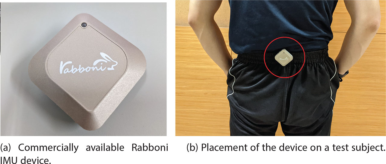
Figure 10:
Rabboni IMU tied on a jumper. (A) Commercially available Rabboni IMU device. (B) Placement of the device on a test subject. IMU, inertial measurement unit.
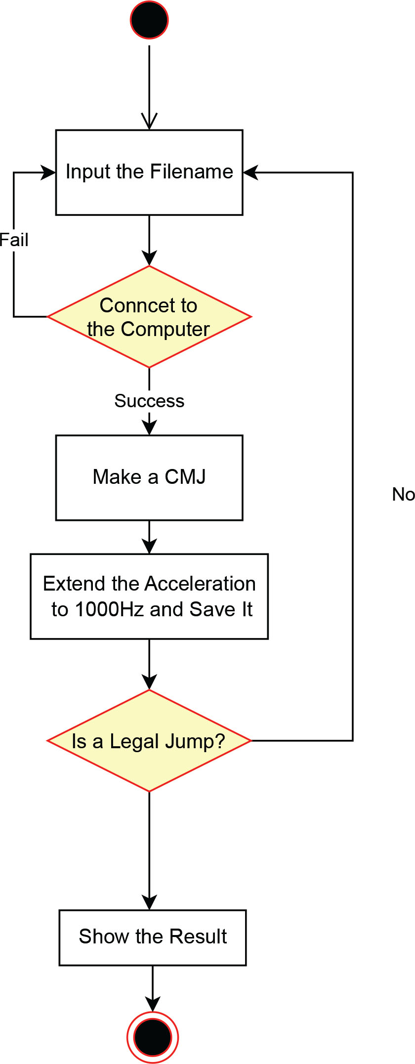
Figure 11:
System architecture and application workflow. CMJ, countermovement jump.
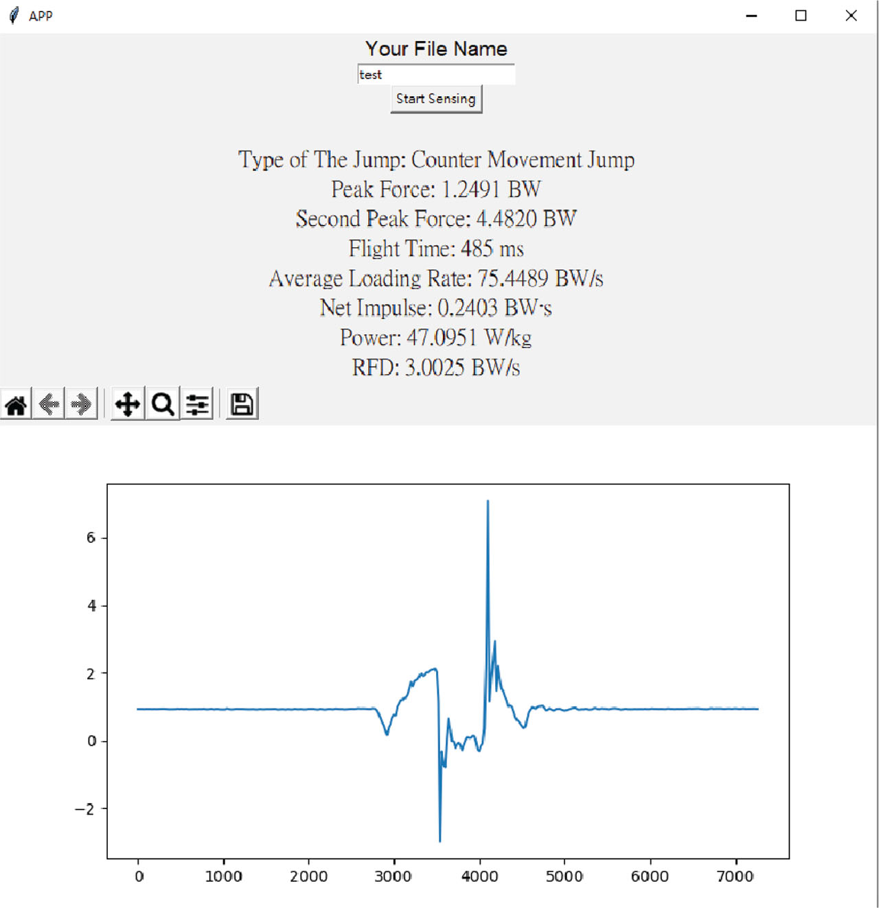
Figure 12.
Prototype system predicting CMJ variable performance in a live test. CMJ, countermovement jump.