
Table 1:
Different synthetic BAF tabular datasets
| Base | Sampled to best represent original dataset |
|---|---|
| Variant I | Has higher group size disparity than base |
| Variant II | Has higher prevalence disparity than base |
| Variant III | Has better separability for one of the groups |
| Variant IV | Has higher prevalence disparity in train |
| Variant V | Has better separability in train for one of the groups |
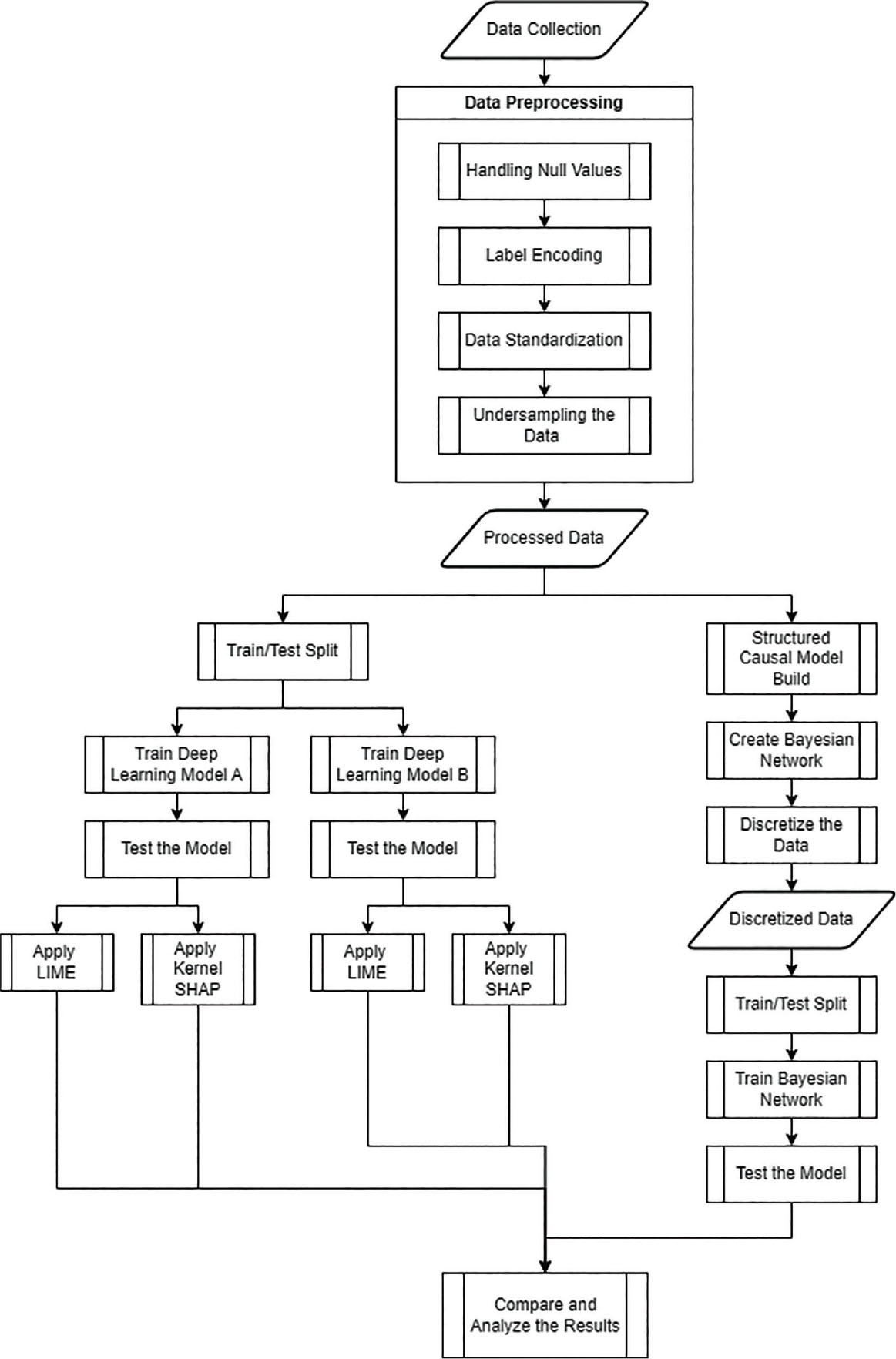
Figure 1:
Research methodology flowchart.
Table 2:
Layers of the first deep learning model
| Model: “sequential” | ||
|---|---|---|
| Layer (type) | Output shape | Param # |
| conv1d (Conv1D) | (None, 29, 64) | 256 |
| max_pooling1d (MaxPooling1D) | (None, 14, 64) | 0 |
| flatten (Flatten) | (None, 896) | 0 |
| dense (Dense) | (None, 64) | 57,408 |
| dense_1 (Dense) | (None, 1) | 65 |
| Total params: 57,729 | ||
| Trainable params: 57,729 | ||
| Non-trainable params: 0 | ||
Table 3:
Layers of the second deep learning model
| Model: “sequential” | ||
|---|---|---|
| Layer (type) | Output shape | Param # |
| conv1d (Conv1D) | (None, 27, 128) | 768 |
| max_pooling1d (MaxPooling1D) | (None, 13, 128) | 0 |
| flatten (Flatten) | (None, 1664) | 0 |
| dense (Dense) | (None, 128) | 213,120 |
| dense_1 (Dense) | (None, 1) | 129 |
| Total params: 214,017 | ||
| Trainable params: 214,017 | ||
| Non-trainable params: 0 | ||
Table 4:
Evaluation matrix of the deep learning models
| Accuracy (%) | Precision (%) | Recall (%) | F1 score (%) | |
|---|---|---|---|---|
| Model 1 | 94.64 | 97.42 | 97.70 | 94.47 |
| Model 2 | 96.34 | 96.06 | 96.64 | 96.35 |
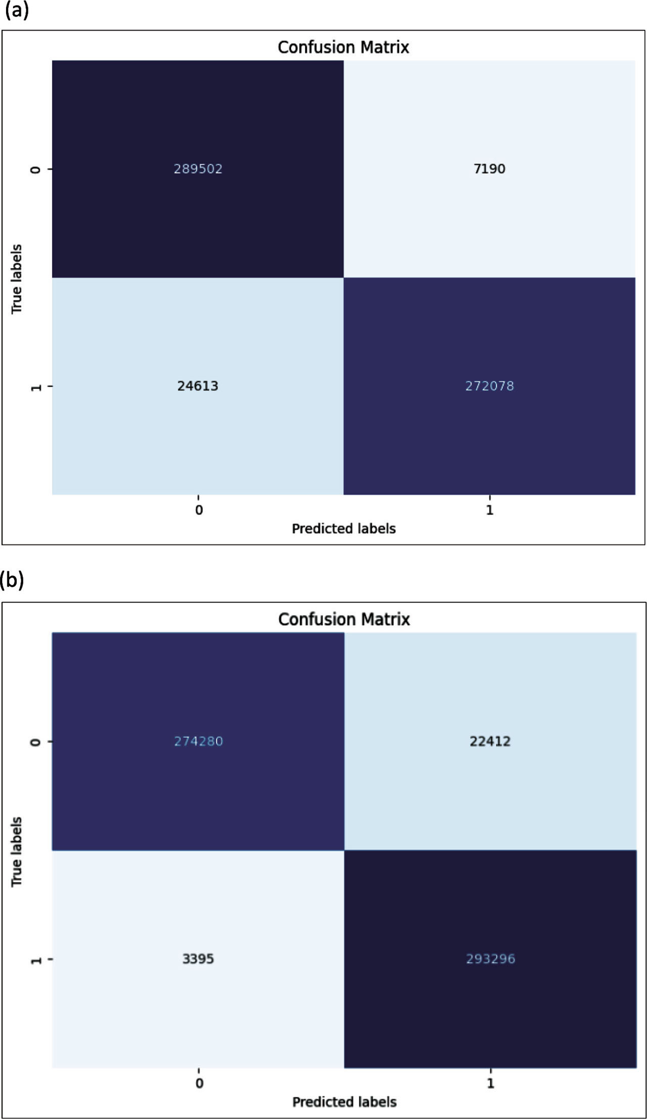
Figure 2:
Confusion matrix of the (A) first and (B) second deep learning models.
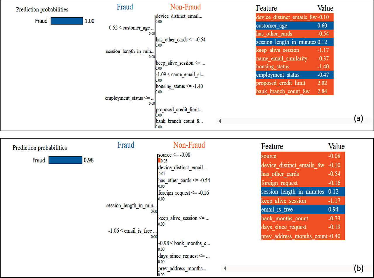
Figure 3:
LIME explanation for single instance for (A) first and (B) second deep learning model. LIME, local interpretable model-agnostic explanations.
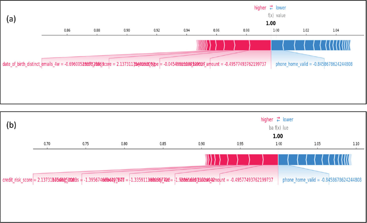
Figure 4:
Force plot of the (A) first deep learning model and (B) second deep learning model.
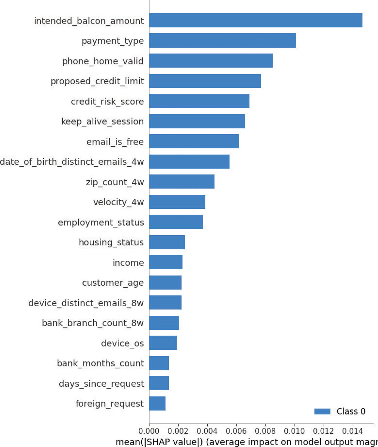
Figure 5:
Summary plot of the first deep learning model.
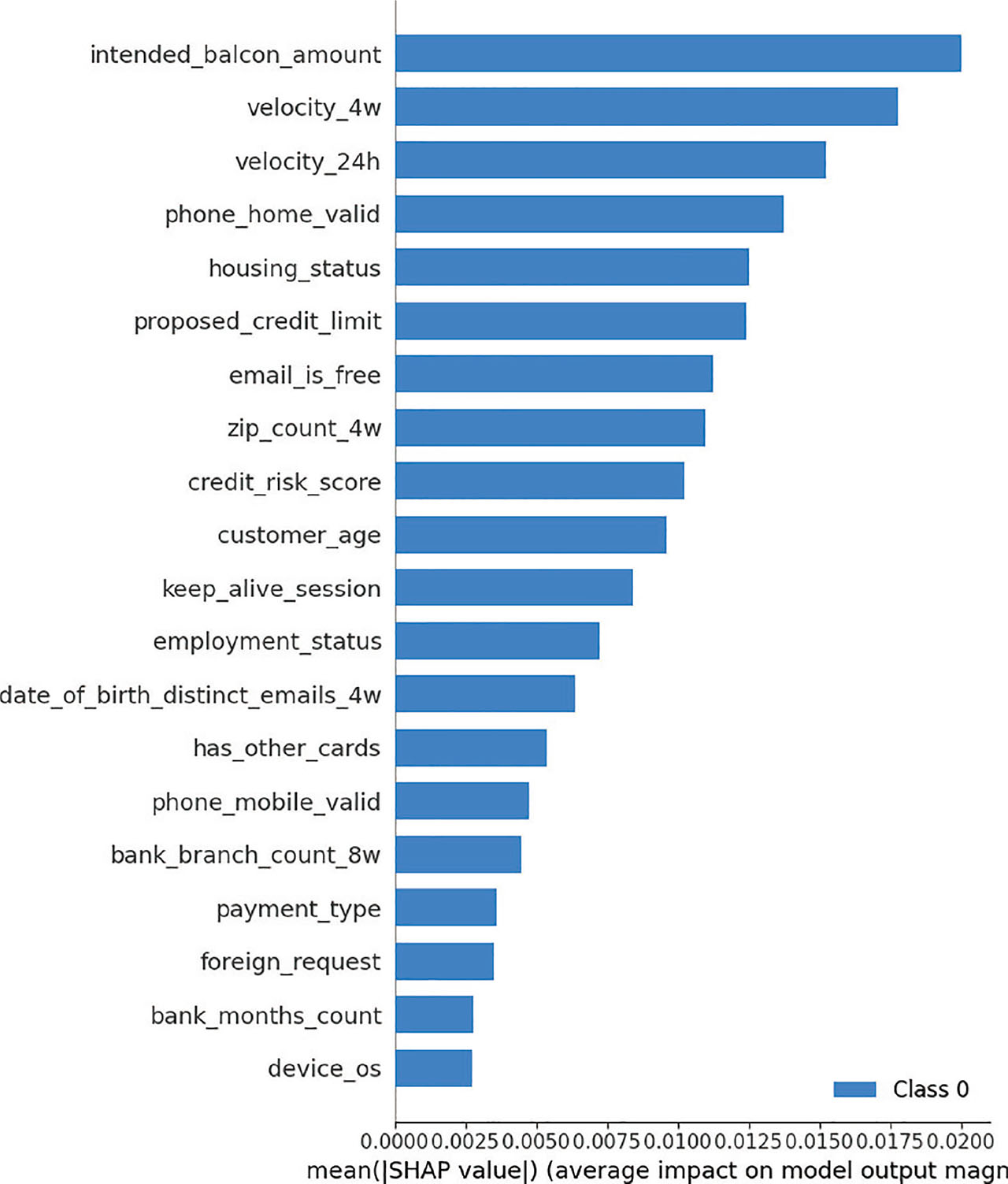
Figure 6:
Summary plot of the second deep learning model.
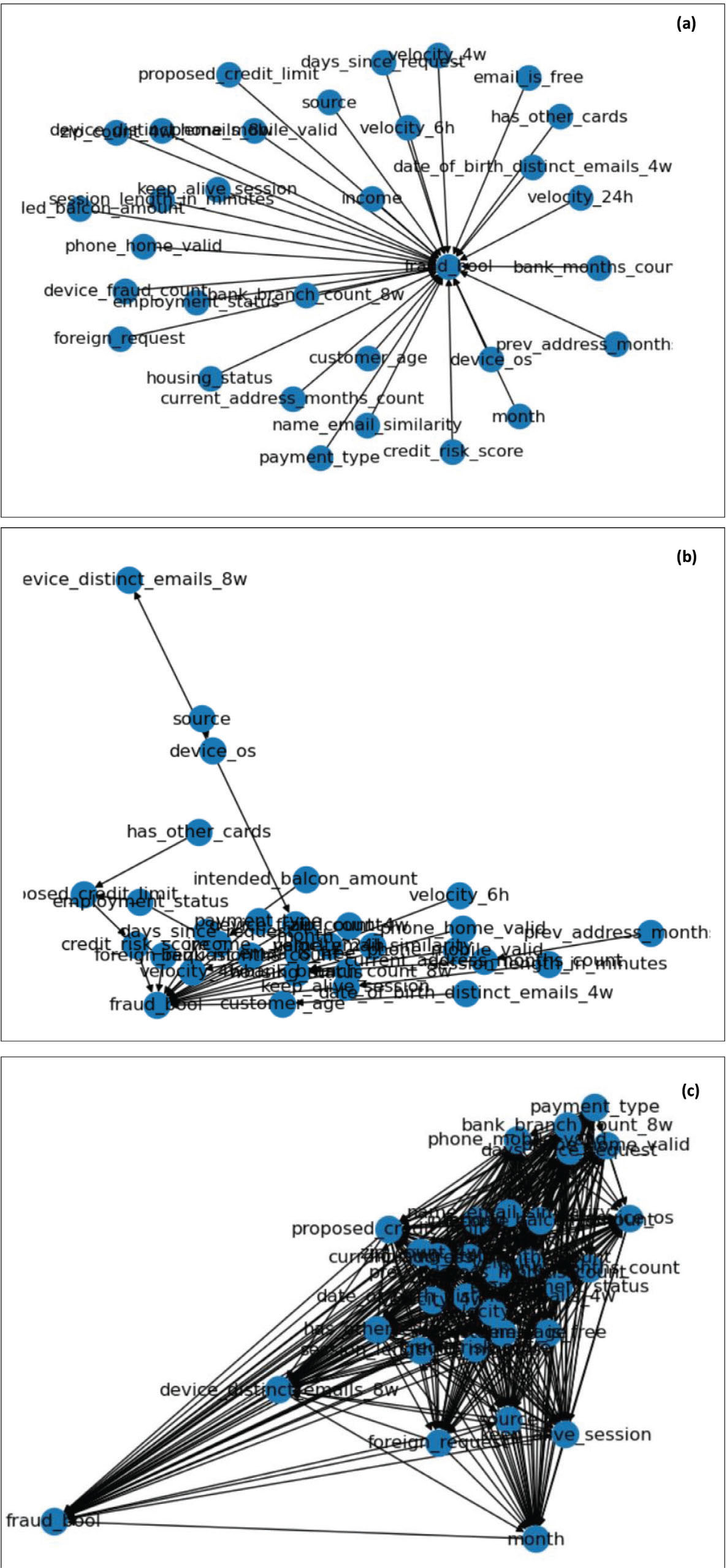
Figure 7:
(A) First SCM; (B) Second SCM; and (C) Third SCM. SCM, structured causal model.
Table 5:
Evaluation matrix of the BNs
| Accuracy (%) | Precision (%) | Recall (%) | F1 score (%) | |
|---|---|---|---|---|
| SCM 1 | 49.32 | 55.66 | 50.79 | 36.59 |
| SCM 2 | 59.27 | 60.50 | 59.02 | 57.67 |
| SCM 3 | 54.94 | 63.00 | 55.65 | 47.95 |
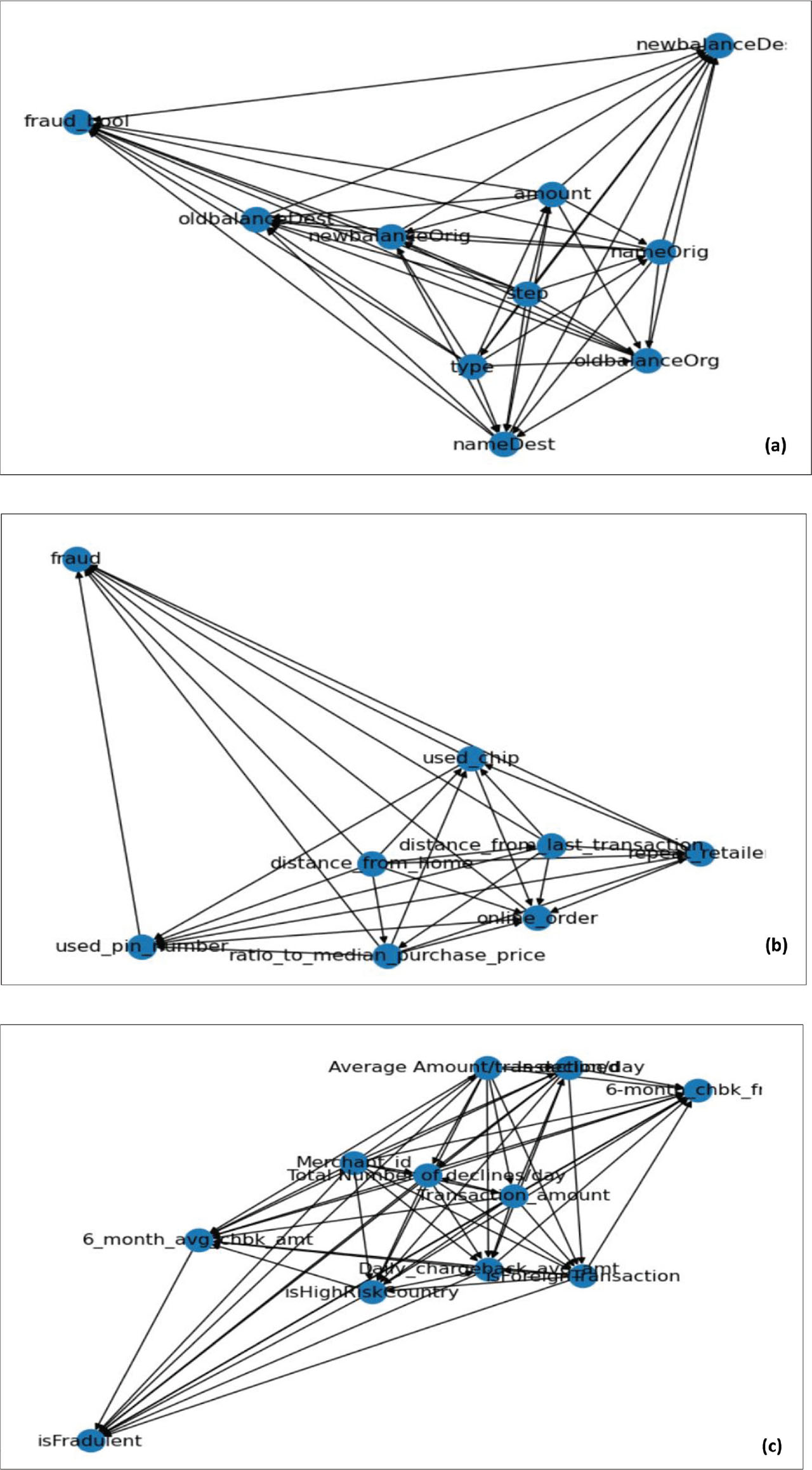
Figure 8:
(A) SCM of the first new data; (B) SCM of the second new data; and (C) SCM of the third new data. SCM, structured causal model.