
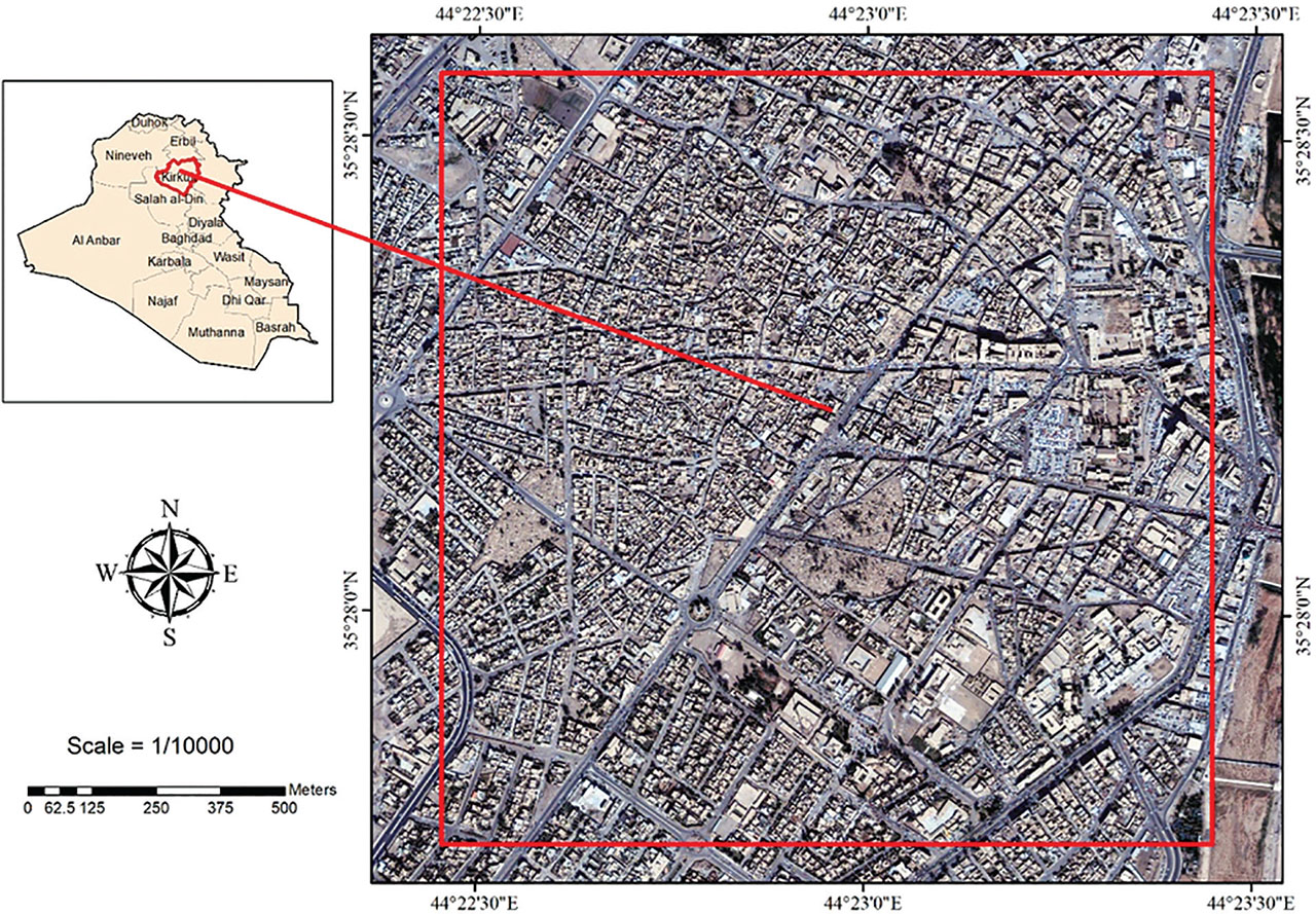
Figure 1:
The study area.
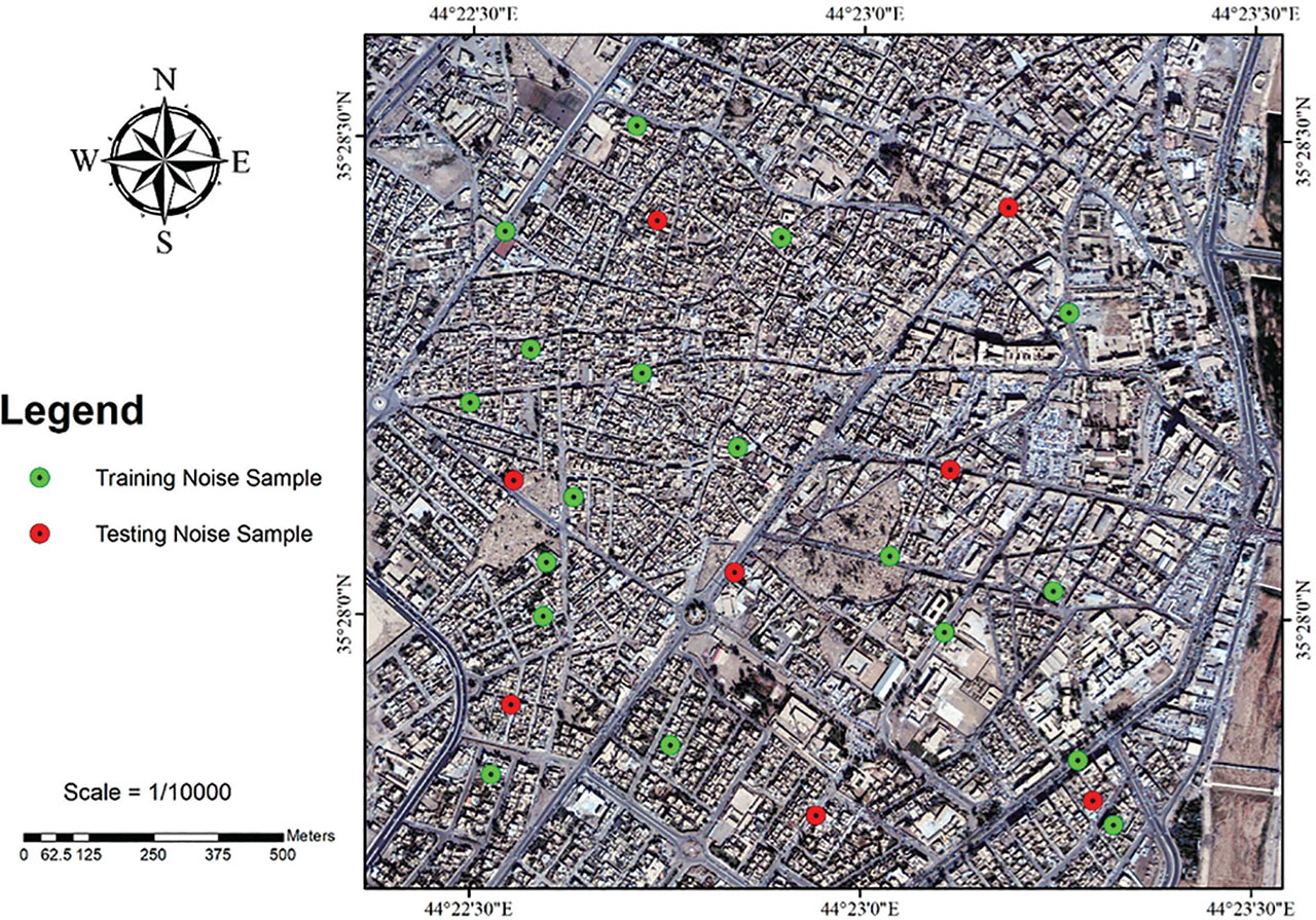
Figure 2:
Training and testing noise samples in the study area.
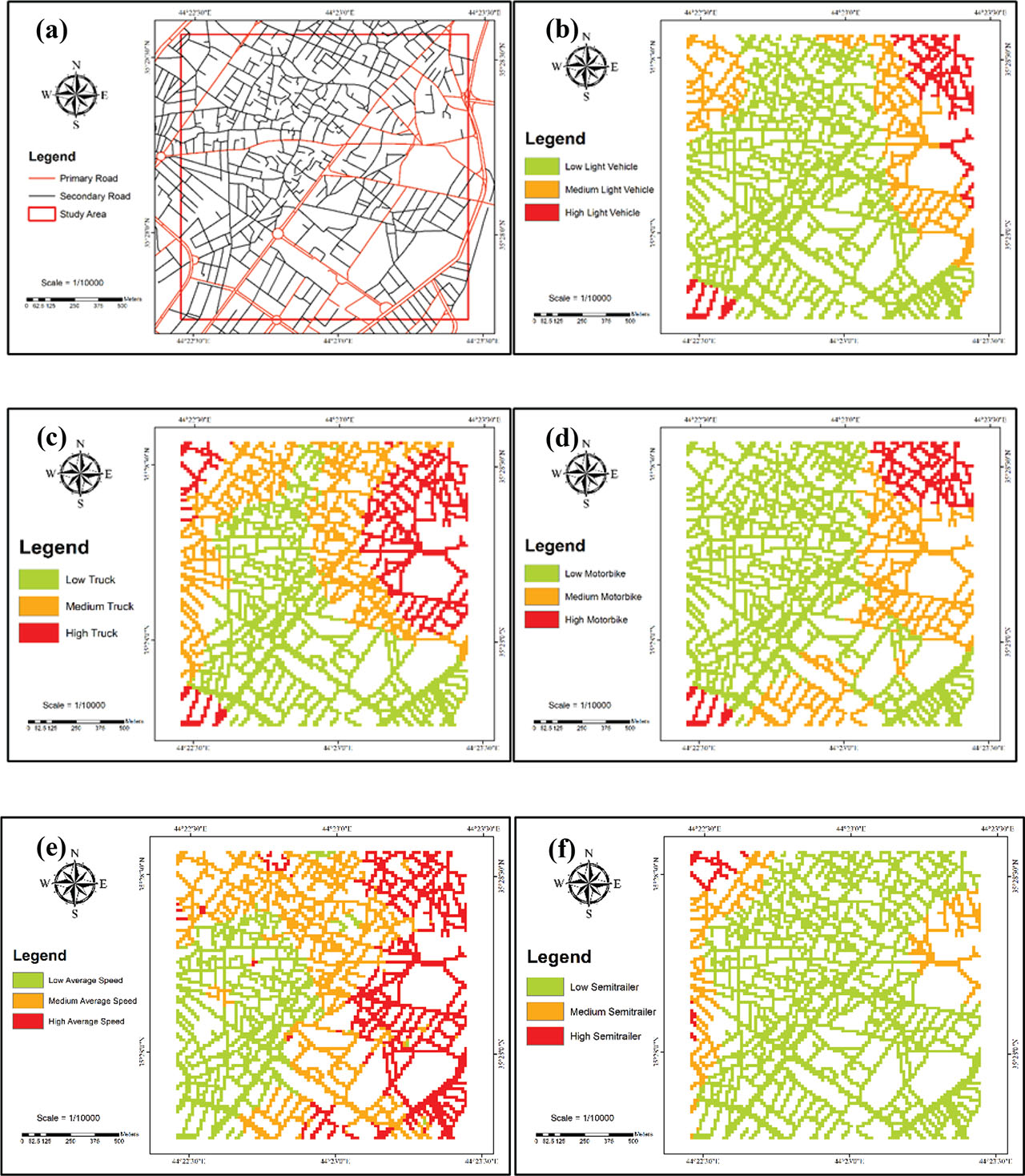
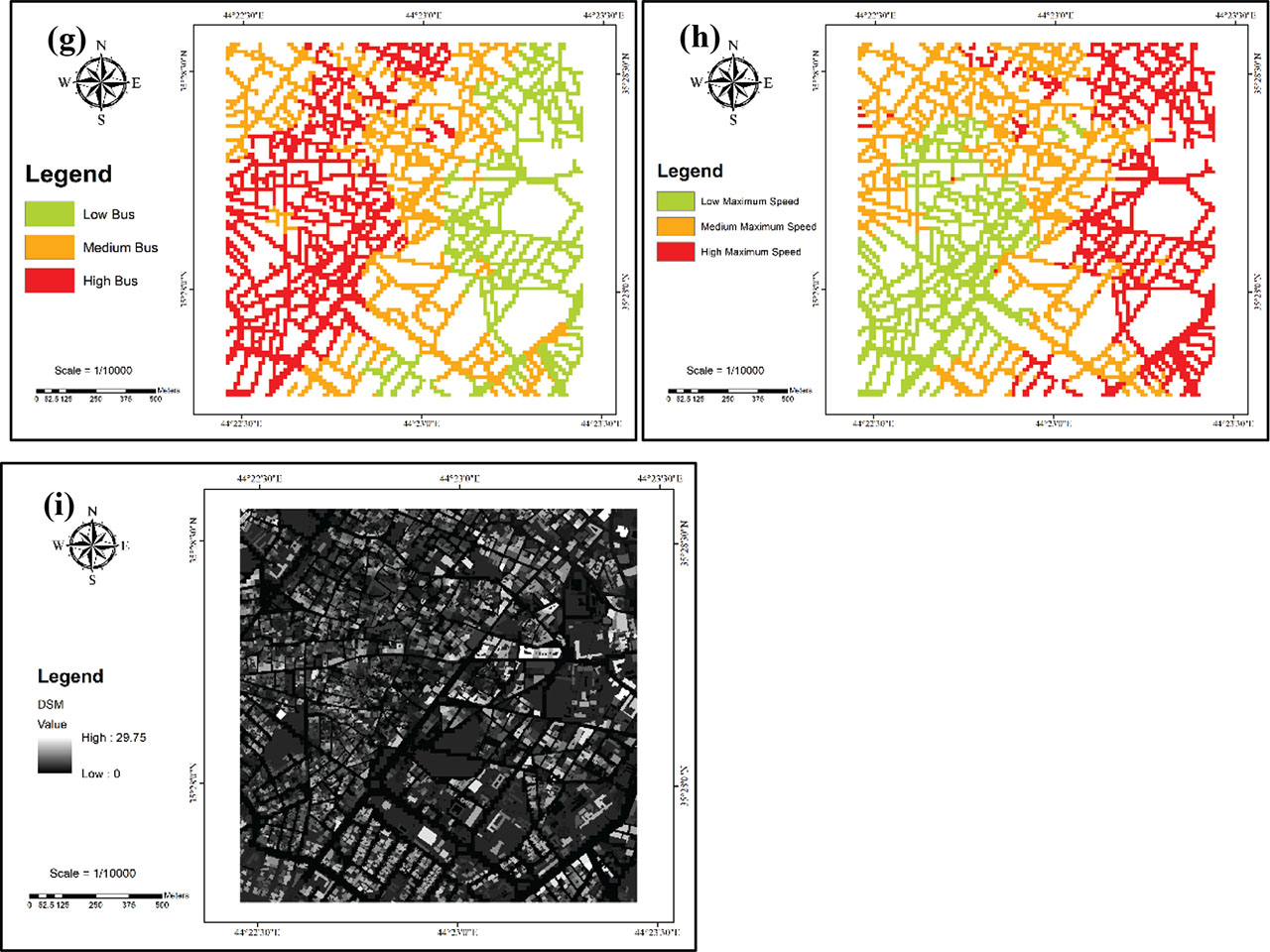
Figure 3:
Different spatial data used in this study: (A) Road networks; (B) Low, medium, and high light vehicles; (C) Low, medium, and high trucks; (D) Low, medium, and high motorbike; (E) Low, medium, and high semitrailer; (F) Low, medium, and high bus; (G) Low, medium, and high average speed; (H) Low, medium, and high maximum speed; (I) DSM. DSM, digital surface model.
Table 1:
Statistical summary of noise predictors of 2D and 3D noise models
| Parameter | Minimum | Maximum | Mean | Deviation |
|---|---|---|---|---|
| Average noise | 28.21 | 83.28 | 47.71 | 20.14 |
| Light vehicle | 0.00 | 354.00 | 20.15 | 70.01 |
| Truck | 0.00 | 92.00 | 8.69 | 22.76 |
| Motorbike | 0.00 | 29.00 | 2.00 | 5.87 |
| Semitrailer | 0.00 | 108.00 | 5.53 | 21.39 |
| Bus | 0.00 | 129.00 | 9.69 | 26.92 |
| DSM | 2.47 | 29.2 | 13.73 | 15.66 |
| Average speed | 0.00 | 49.64 | 11.65 | 17.02 |
| Maximum speed | 0.00 | 66.00 | 13.69 | 21.57 |
| Distance from high volume of light vehicle | 0.00 | 1079.08 | 432.70 | 261.98 |
| Distance from medium volume of light vehicle | 0.00 | 1002.72 | 252.37 | 239.22 |
| Distance from low volume of light vehicle | 0.00 | 539.36 | 58.45 | 103.52 |
| Distance from high volume of truck | 0.00 | 628.94 | 220.19 | 164.74 |
| Distance from medium volume of truck | 0.00 | 594.40 | 119.59 | 129.21 |
| Distance from low volume of truck | 0.00 | 738.88 | 120.67 | 161.98 |
| Distance from high volume of motorbike | 0.00 | 1157.50 | 468.80 | 268.63 |
| Distance from medium volume of motorbike | 0.00 | 926.08 | 243.85 | 233.62 |
| Distance from low volume of motorbike | 0.00 | 569.75 | 65.09 | 114.28 |
| Distance from high volume of semitrailer | 0.00 | 1549.70 | 636.87 | 378.83 |
| Distance from medium volume of semitrailer | 0.00 | 849.06 | 250.78 | 191.34 |
| Distance from low volume of semitrailer | 0.00 | 379.29 | 25.43 | 47.44 |
| Distance from high volume of bus | 0.00 | 910.39 | 158.78 | 208.53 |
| Distance from medium volume of bus | 0.00 | 445.29 | 84.82 | 88.49 |
| Distance from low volume of bus | 0.00 | 1059.13 | 295.93 | 272.59 |
| Distance from high volume of average speed | 0.00 | 666.25 | 141.29 | 137.27 |
| Distance from medium volume of average speed | 0.00 | 406.50 | 78.55 | 81.38 |
| Distance from low volume of average speed | 0.00 | 652.80 | 117.52 | 129.15 |
| Distance from high volume of maximum speed | 0.00 | 722.50 | 170.70 | 178.77 |
| Distance from medium volume of maximum speed | 0.00 | 442.07 | 75.57 | 84.09 |
| Distance from low volume of maximum speed | 0.00 | 829.62 | 179.87 | 195.56 |
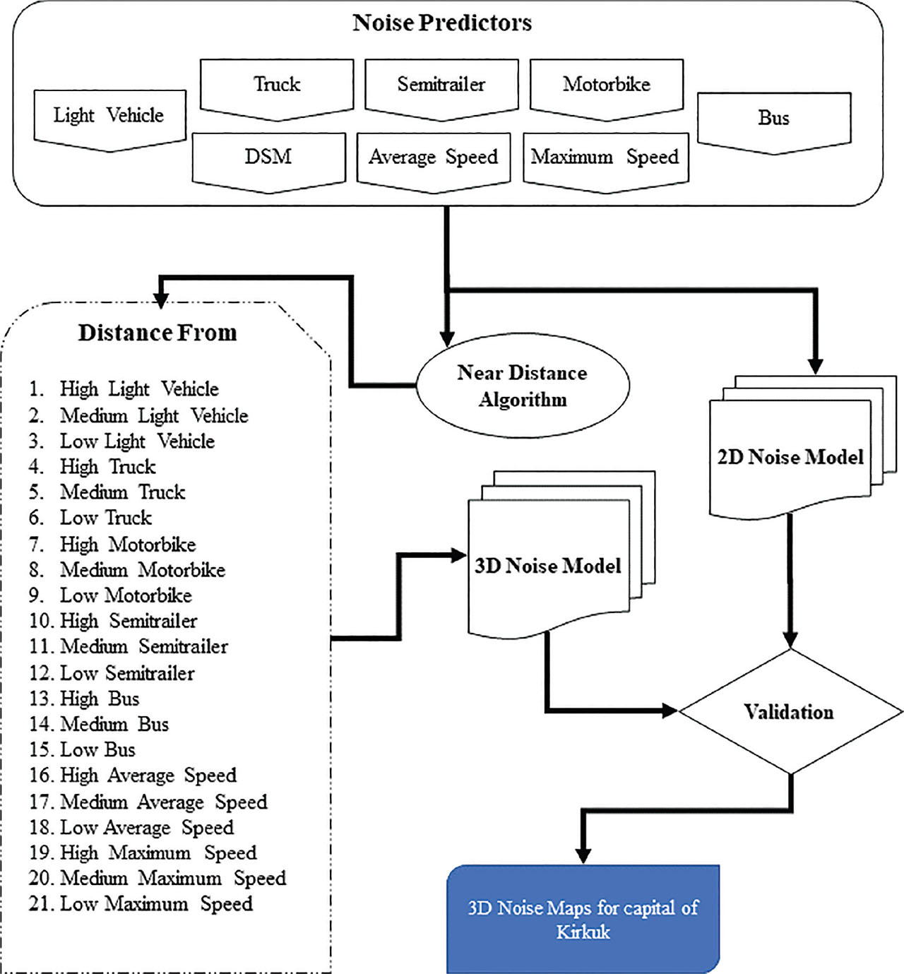
Figure 4:
Methodology used in this work.
Table 2:
Hyperparameters of the proposed model for traffic noise prediction and their search space used for fine-tuning
| Hyperparameters | Search domain |
|---|---|
| Type of network | {multilayer perceptron (MLP)} |
| Number of hidden units | (3–30) |
| Training algorithm | {BFGS, RBFT} |
| Hidden and output activation | {Identity, Logistic, Tanh, Exponential, Gaussian} |
| Learning rate | (0.01–0.9) by step of 0.05 |
| Momentum | (0.1–0.9) by step of 0.1 |
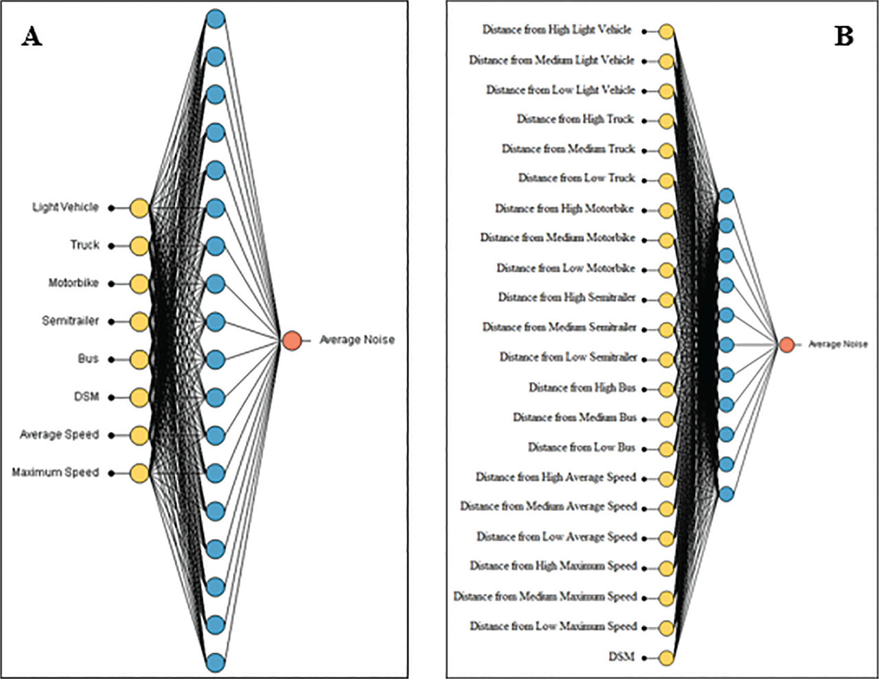
Figure 5:
(A) Architecture of ANN of 2D traffic noise prediction (8-18-1), (B) architecture of ANN of 3D traffic noise prediction (22-11-1). 2D, two-dimensional; 3D, three-dimensional; ANN, artificial neural network.
Table 3:
Shows the hidden and output activation of the ANN model
| Model | Hyperparameter | Identity | Logistic | Tanh | Exponential | Gaussian |
|---|---|---|---|---|---|---|
| 2D Noise Model | Hidden and output activation | 0.003 | 0.0248 | 0.1892 | 2.0043 | 0.2373 |
| 3D Noise Model | 0.0805 | 0.058 | 0.3584 | 1.2066 | 0.1166 |
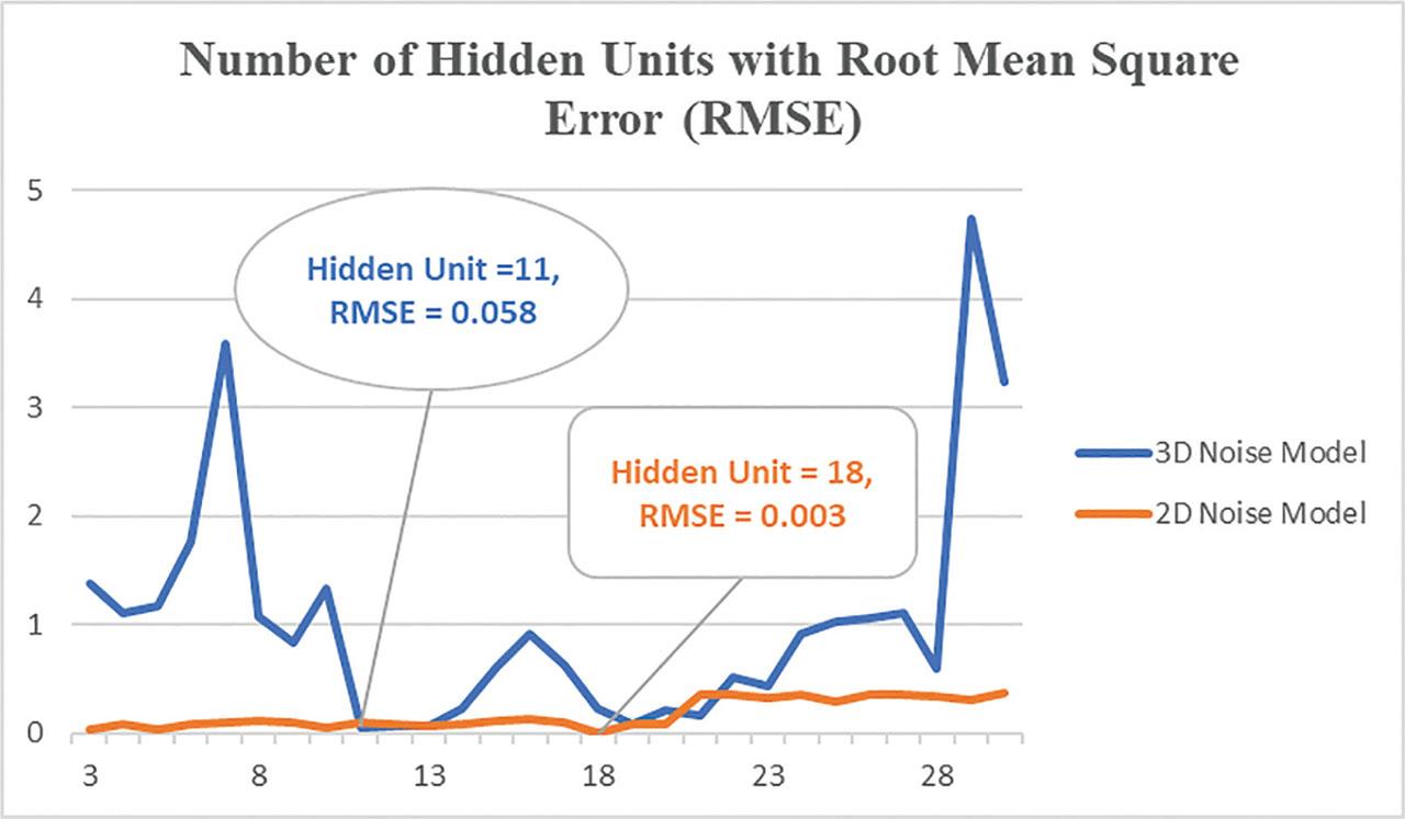
Figure 6:
Number of hidden units with RMSE for 2D and 3D noise model prediction. 2D, two-dimensional; 3D, three-dimensional; RMSE, root mean square error.
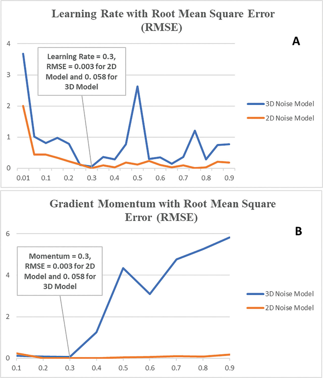
Figure 7:
(A) Learning rate and (B) gradient momentum with RMSE for 2D and 3D noise model prediction. 2D, two-dimensional; 3D, three-dimensional; RMSE, root mean square error.
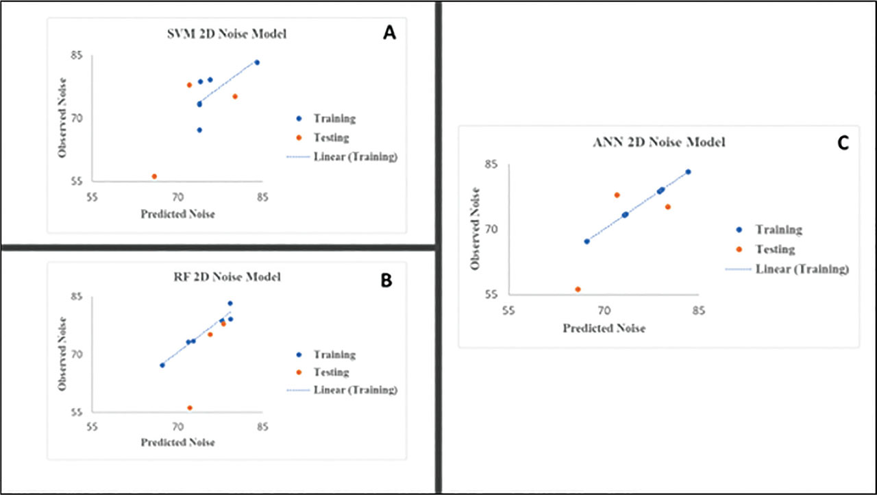
Figure 8:
The correlation of training and testing noise models between observed and predicted of 2D traffic noise for (A) SVM, (B) RF, and (C) ANN models. 2D, two-dimensional; ANN, artificial neural network; RF, random forest; SVM, support vector machine.
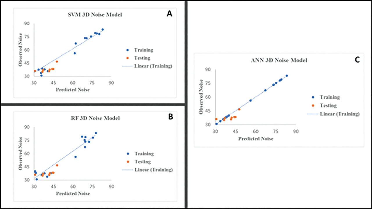
Figure 9:
The correlation of training and testing noise models between observed and predicted of 3D traffic noise for (A) SVM, (B), RF, and (C) ANN models. 3D, three-dimensional; ANN, artificial neural network; RF, random forest; SVM, support vector machine.
Table 4:
Performance of models such as ANN, SVM, and RF for 2D and 3D noise models
| Model | Type of model | Training (R) | Testing (R) | Training (R2) | Testing (R2) | Training (RMSE) | Testing (RMSE) |
|---|---|---|---|---|---|---|---|
| 2D Noise Model | ANN | 1.00 | 0.87 | 1.00 | 0.75 | 0.003 | 7.14 |
| SVM | 0.85 | 0.81 | 0.72 | 0.65 | 3.60 | 10.34 | |
| RF | 0.98 | 0.82 | 0.97 | 0.68 | 1.82 | 9.83 | |
| 3D Noise Model | ANN | 1.00 | 0.82 | 1.00 | 0.68 | 0.058 | 4.46 |
| SVM | 0.98 | 0.77 | 0.96 | 0.60 | 6.16 | 4.75 | |
| RF | 0.98 | 0.80 | 0.96 | 0.64 | 6.00 | 4.50 |
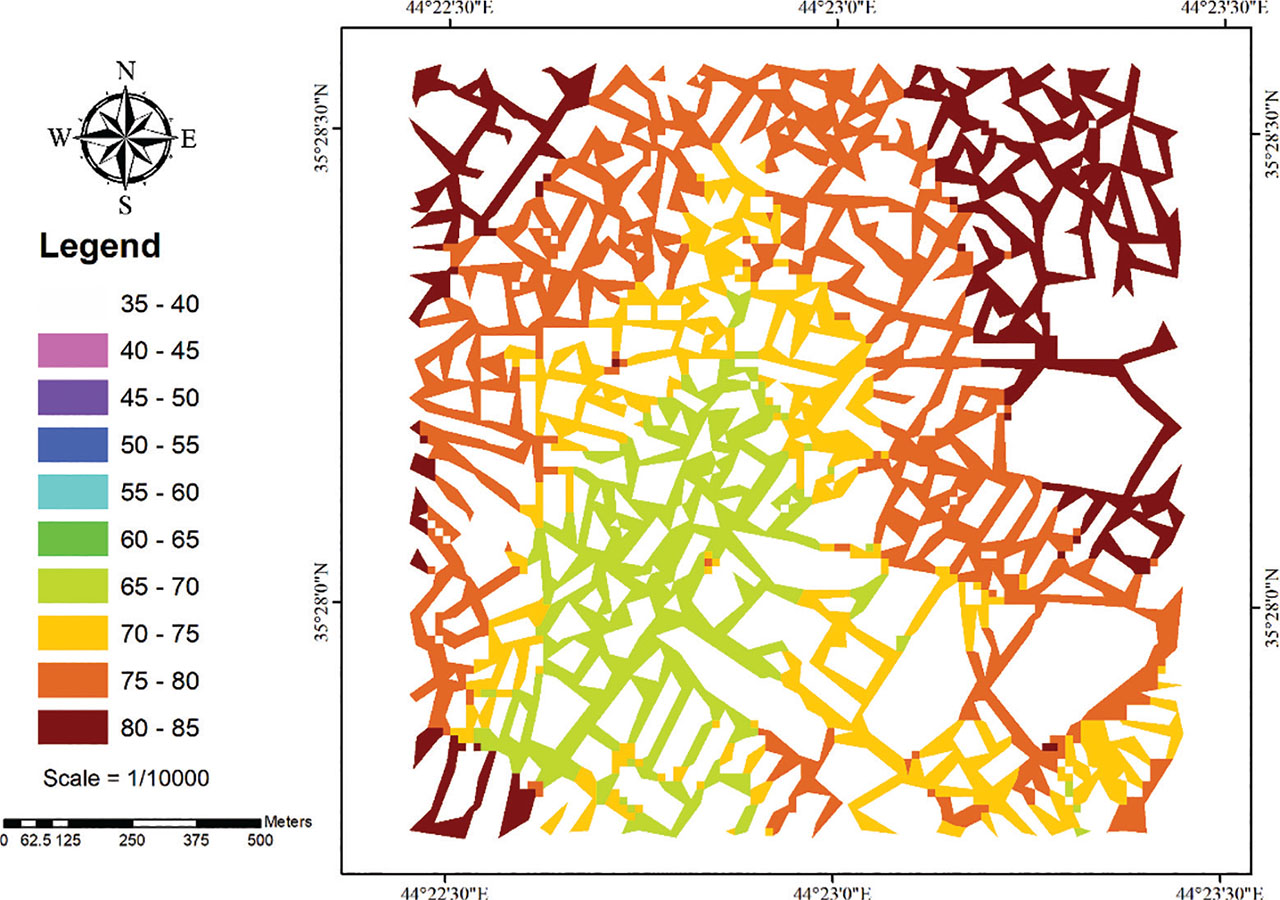
Figure 10:
2D average noise prediction map for roads in the study area from 2D ANN noise model. 2D, two-dimensional; ANN, artificial neural network.
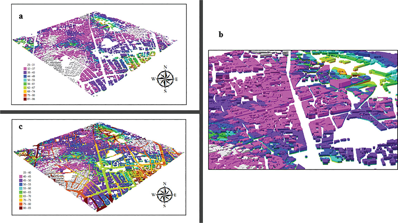
Figure 11:
(A) 3D average noise prediction map for building in the study area from the 3D noise model, (B) average noise prediction map for building in the study area from the 3D noise model for part of the study area, (C) average noise prediction map for roads and building at the study area through combined 2D and 3D model maps. 2D, two-dimensional; 3D, three-dimensional.