
Table 1.
Comparison with the previously reported works.
| Material | Method | Range (μM) | LoD (μM) | Ref. |
|---|---|---|---|---|
| CoPCNF/GCE | CV | 75–770 | 46 | [22] |
| CEC | CV | 100–1000 | 9 | [23] |
| Mercury/Platinum | CSSV | 1–20 | 0.25 | [24] |
| HMDE | SWP | 0.2–83 | 0.1 | [25] |
| HMDE | DPCSV | 3–20 | 2 | [26] |
| BDD | CV | 20–100 | 0.8 | [27] |
| GCE | SWV | 3–120 | 0.10 | [28] |
| LIG/MB | CA/CV | 0.5–500 | 0.435 | This work |
[i] BDD, boron-doped diamond electrode; CA, chronoamperometry; CEC, carbon epoxy composite; CoPCNF, Cobalt pentacyanonitrosylferrate; CSSV, cathodic stripping sweep voltammetry; CV, cyclic voltammetry; DPCSV, differential pulse cathodic stripping voltammetry; GCE, glassy carbon electrode; HMDE, hanging mercury drop electrode; LIG, laser-induced graphene; MB, methylene blue; SWP, square wave polarography.
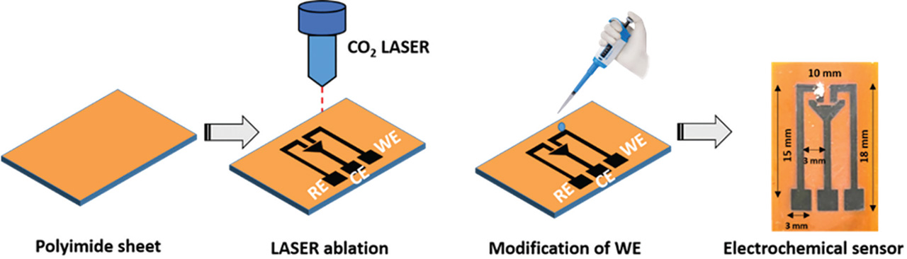
Scheme I:
Schematic of the electrochemical sensor fabrication with the real image of the sensor.
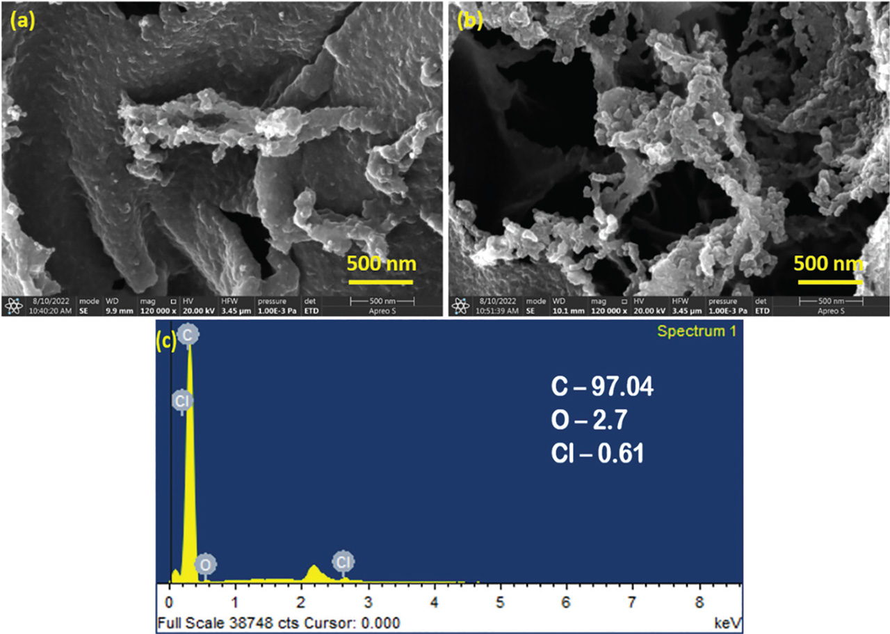
Figure 1:
(a) SEM image of bare LIG (b) modified with MB (c) EDX analysis. EDX, energy dispersive X-ray; LIG, laser-induced graphene; MB, methylene blue; SEM, scanning electron microscopy.
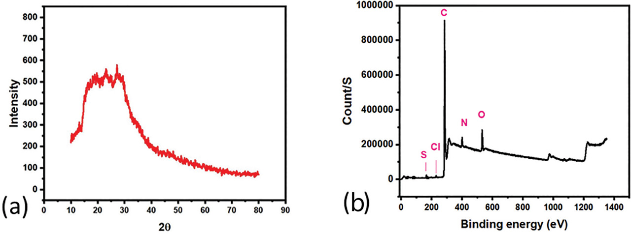
Figure 2:
(a) XRD of the LIG/MB (b) XPS of the LIG/MB modification. LIG, laser-induced graphene; MB, methylene blue; XRD, X-ray diffraction; XPS, X-ray photoelectron scattering.
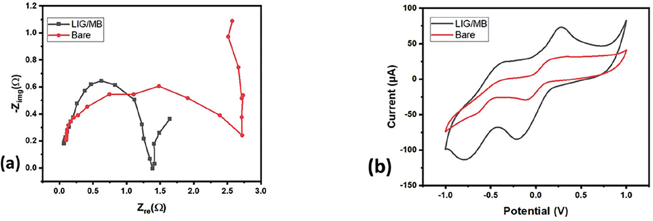
Figure 3:
(a) EIS of bare LIG and LIG/MB, (b) Comparative CV response of LIG and LIG/MB with the potassium ferricyanide–KCl solution for 50 mV/S, n = 4 (number of cycle). CV, cyclic voltammetry; EIS, electrochemical impedance spectroscopy; LIG, laser-induced graphene; MB, methylene blue.
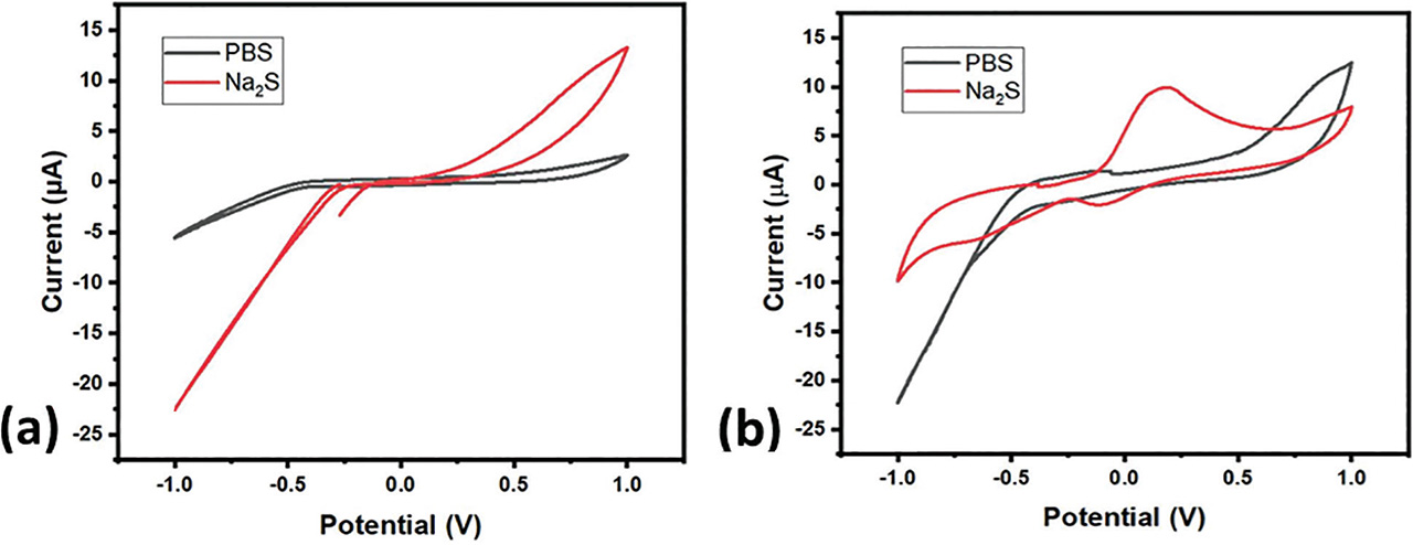
Figure 4:
(a) Comparative CV of bare LIG in pH7 PBS and 1 mM Na2S at 10 mV/S for n = 4, (b) Comparative CV of LIG/MB in (pH = 7) PBS and 1 mM Na2S at 10 mV/S for n = 4. CV, cyclic voltammetry; LIG, laser-induced graphene; MB, methylene blue; PBS, phosphate buffer solution.
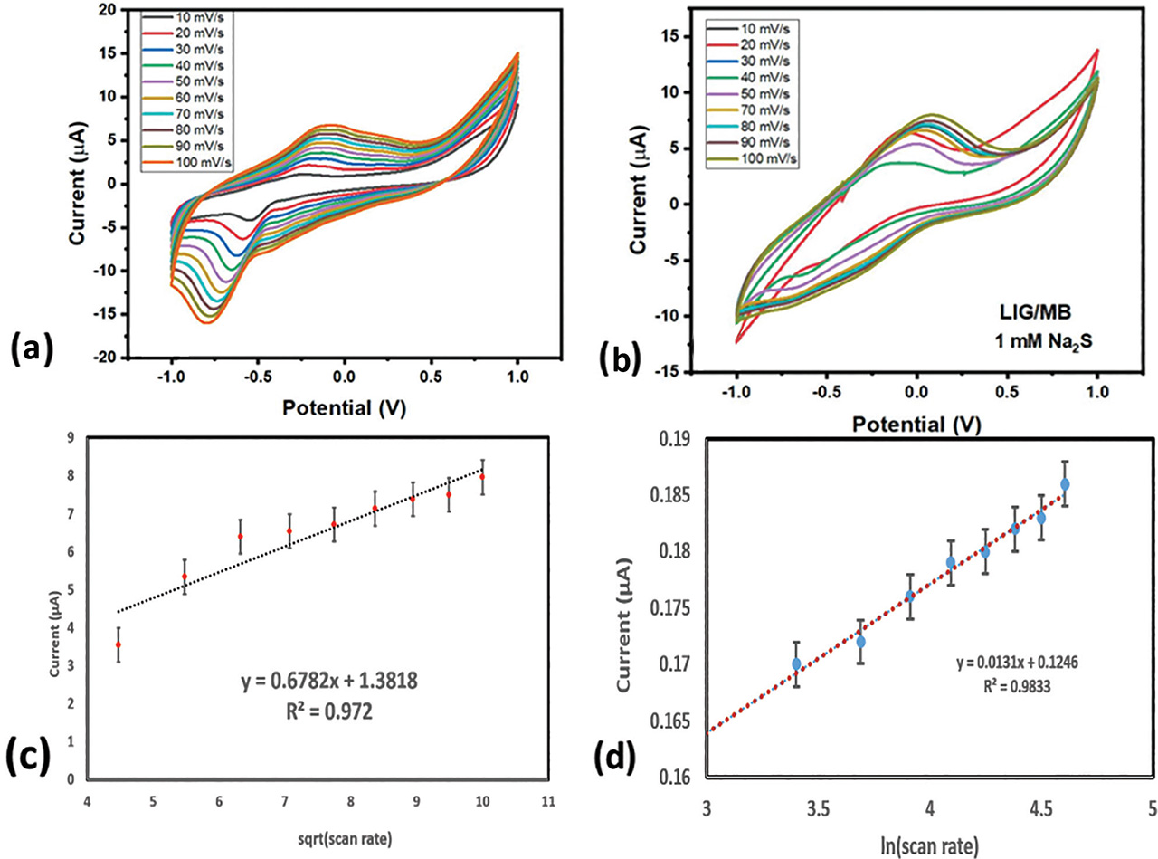
Figure 5:
(a) Scan rate of 0.1 M PBS (pH = 7.4) on LIG/MB electrochemical sensor, (b) Scan rate test of 1 mM Na2S on LIG/MB electrochemical sensor, (c) Scan rate calibration curve (Ipa vs. sqrt(ν)) (d) Laviron plot of the LIG/MB electrochemical sensor from the scan rate plot. LIG, laser-induced graphene; MB, methylene blue; PBS, phosphate buffer solution.
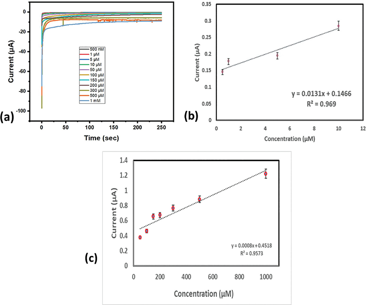
Figure 6:
(a) Concentration analysis on LIG/MB–based electrochemical sensor (b) calibration curve of the concentration analysis Ipa vs. concentration. Two linear ranges can be observed. LIG, laser-induced graphene; MB, methylene blue.
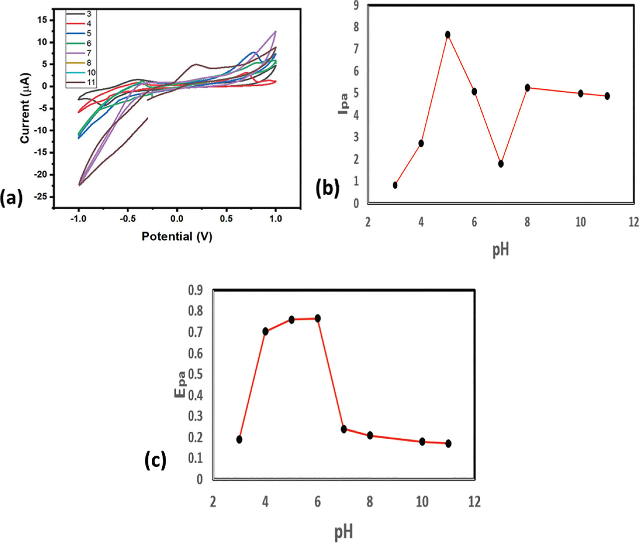
Figure 7
(a) pH analysis of PBS on the LIG/MB electrochemical sensor ranging from 3 to 11 pH (b) Ipa vs. pH (c) Epa vs. pH. LIG, laser-induced graphene; MB, methylene blue; PBS, phosphate buffer solution.
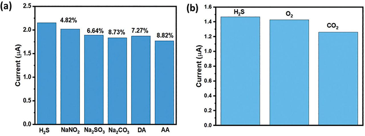
Figure 8:
Interference effect analysis (a) with the direct interfering analyte (b) with the gases.
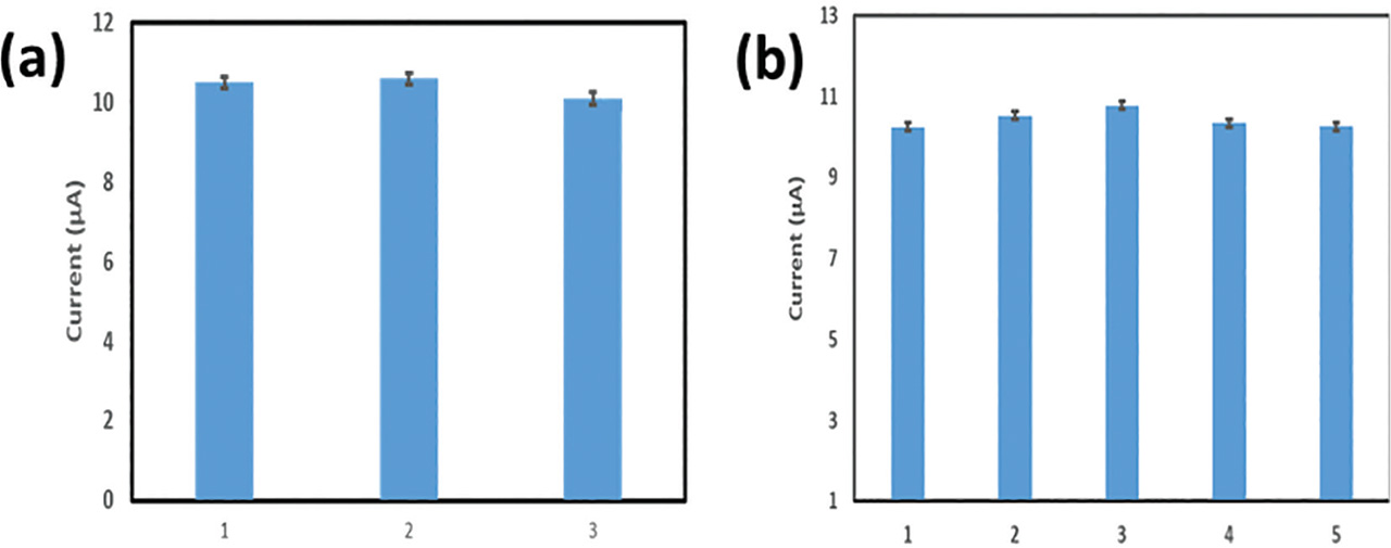
Figure 9:
(a) Repeatability and (b) reproducibility of the fabricated electrochemical.
Table 2.
Real sample analysis.
| Source of Lake Water | S. No. | Added (μM) | Found (μM) | Recovery (%) | RSD |
|---|---|---|---|---|---|
| Shameerpet Lake | 1 | 10 | 9.866667 | 98.7 | 2.055076 |
| 2 | 50 | 49.26667 | 98.6 | 4.72582 | |
| 3 | 100 | 99.3 | 99.3 | 2.64575 | |
| Hussain Sagar Lake | 1 | 10 | 9.8 | 98 | 1.37477 |
| 2 | 50 | 49.71333 | 99.44 | 2.41316 | |
| 3 | 100 | 99.89 | 99.89 | 3.6056 | |
| Kapra Lake | 1 | 10 | 9.843333 | 98.5 | 1.76376 |
| 2 | 50 | 49.07667 | 98.2 | 4.45459 | |
| 3 | 100 | 99.61 | 99.61 | 2.91376 |
[i] RSD, relative standard deviation.
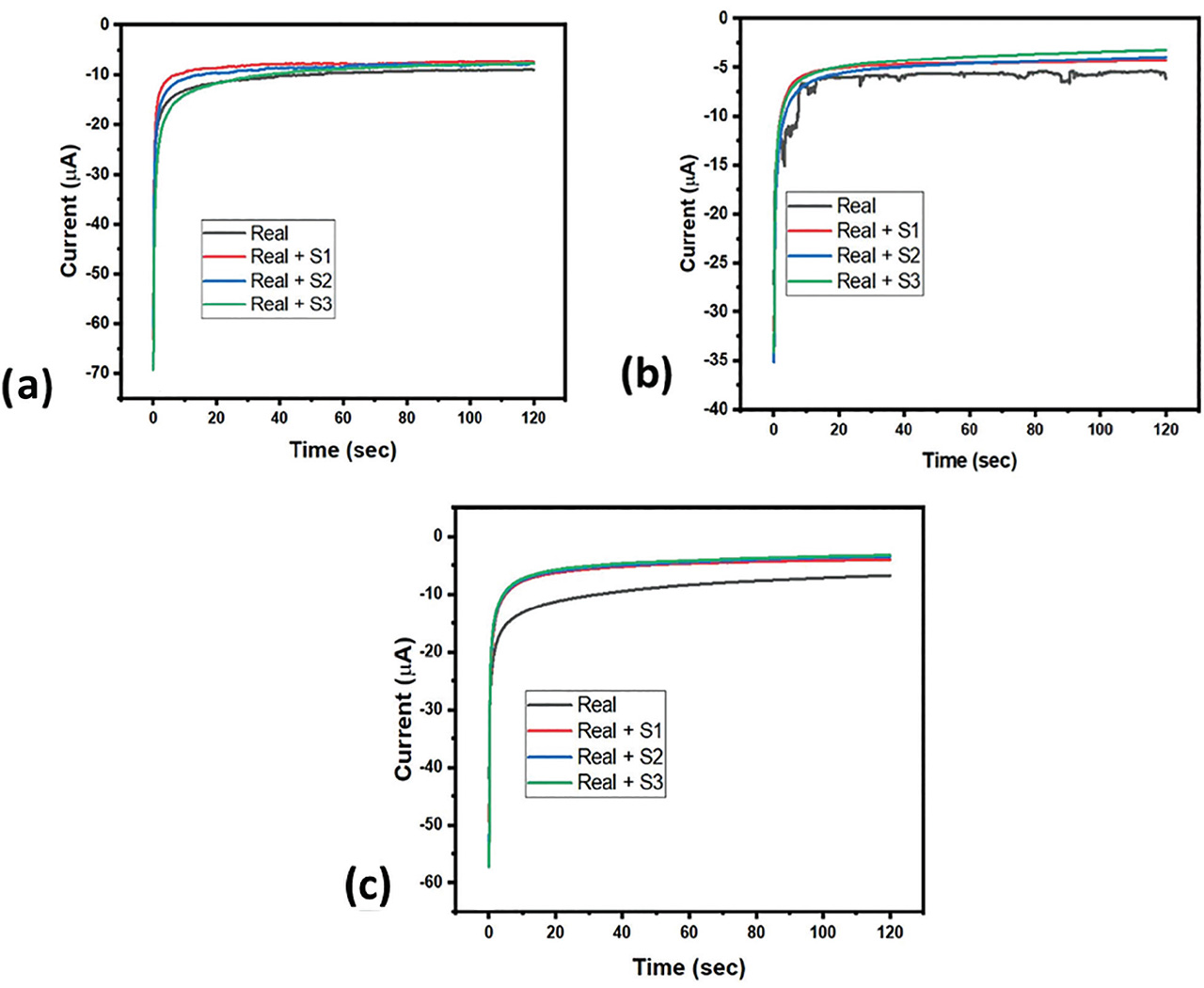
Figure 10:
Real Sample analysis of (a) Kapra Lake, (b) Hussain Sagar Lake, (c) Shameerpet Lake.