
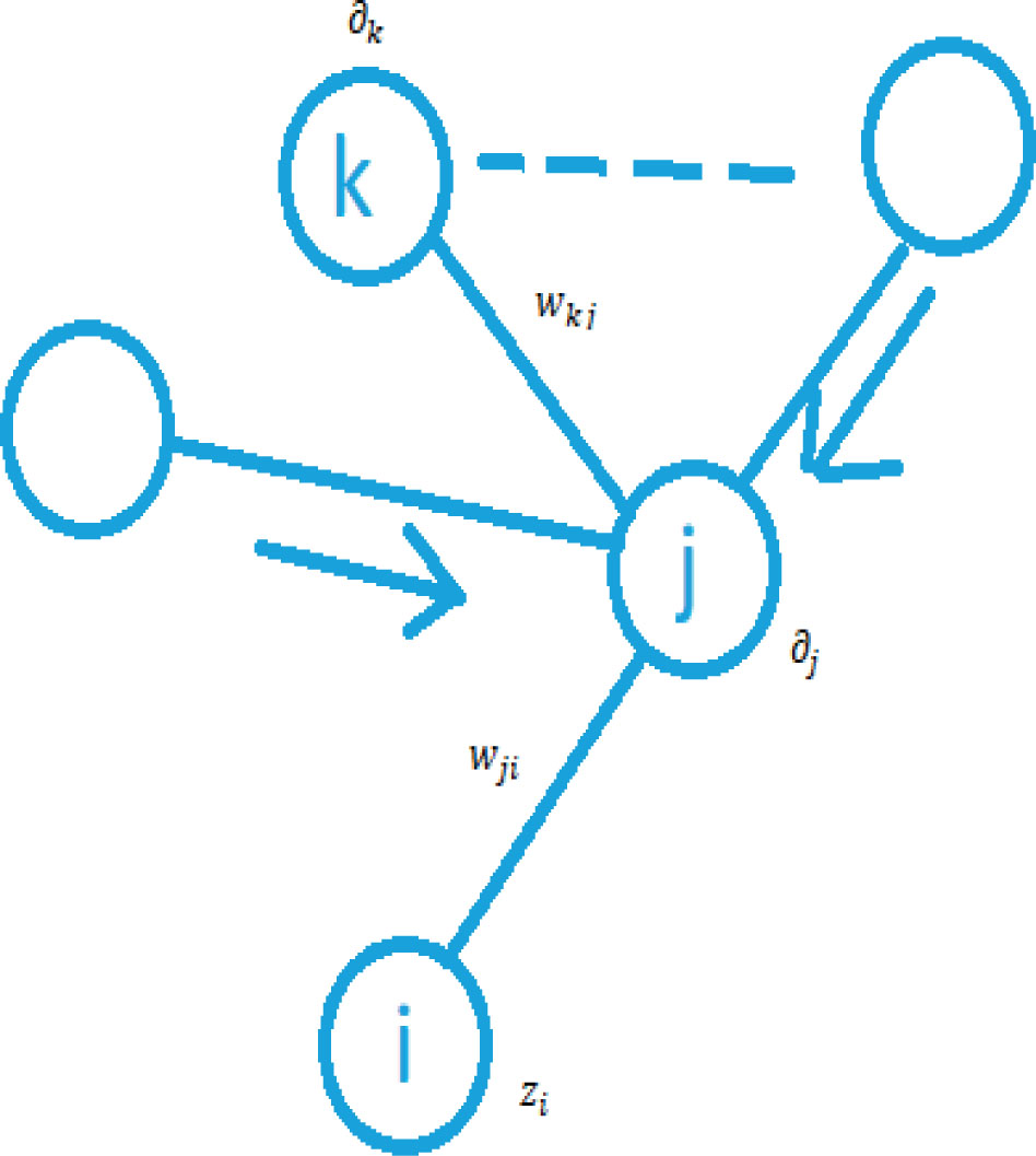
Figure 1:
Schematic illustration of computation of ∂j for hidden unit j with the help of back propagation.
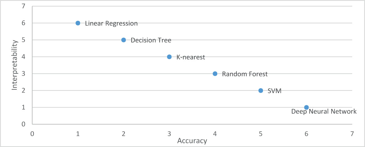
Figure 2:
The accuracy of deep learning models is higher, but their interpretability is low compared to other ML models.
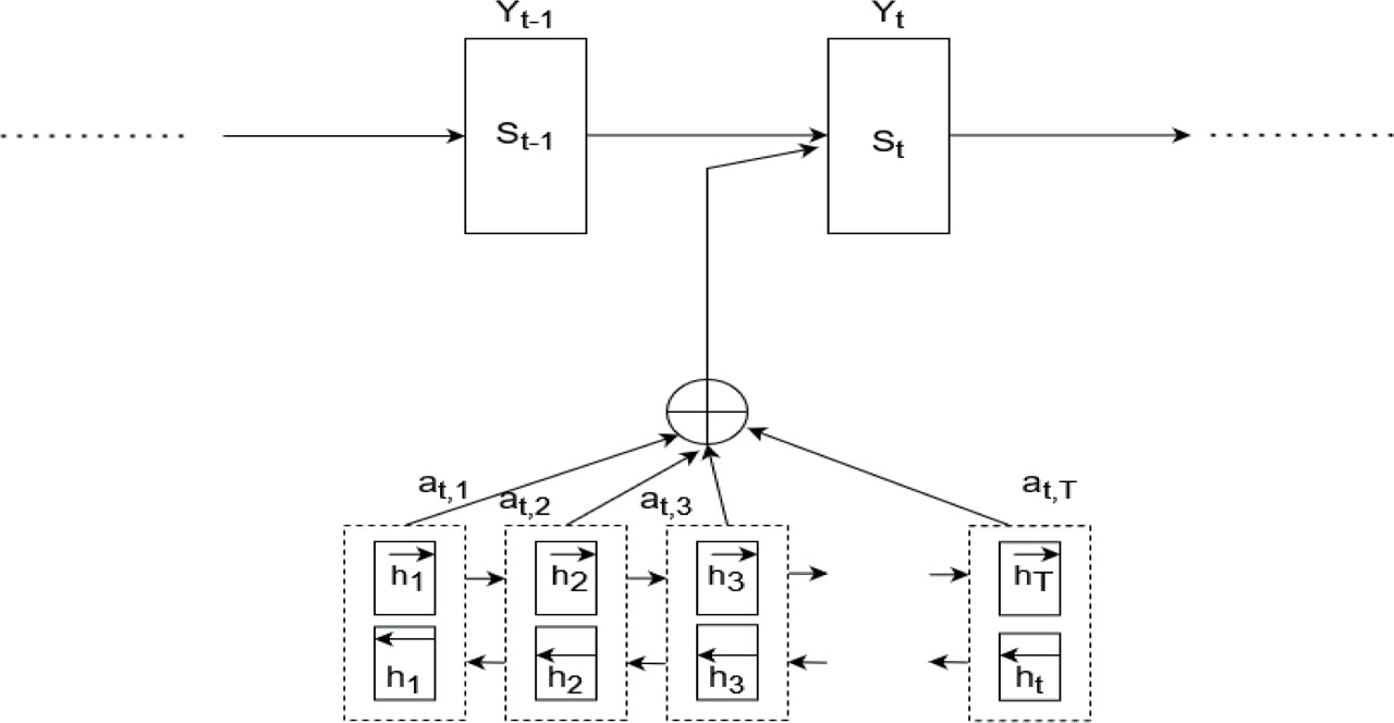
Figure 3:
Schematic representation of bidirectional RNN (Source: Bahdanau et al. [26]).
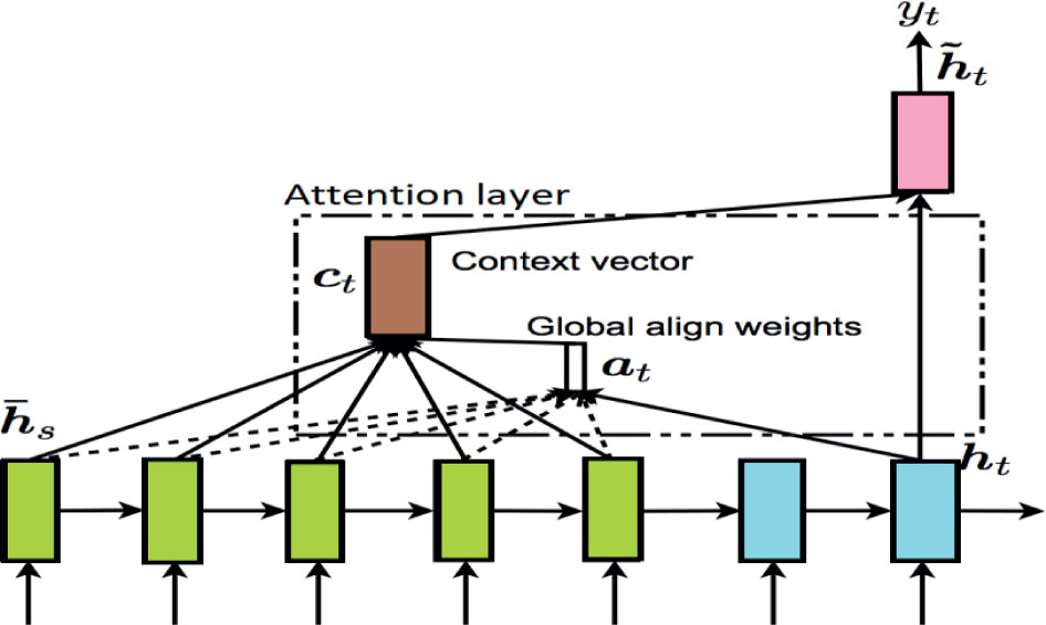
Figure 4:
RNN with global attention.
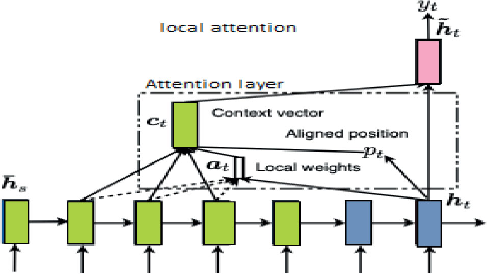
Figure 5:
RNN with local attention.
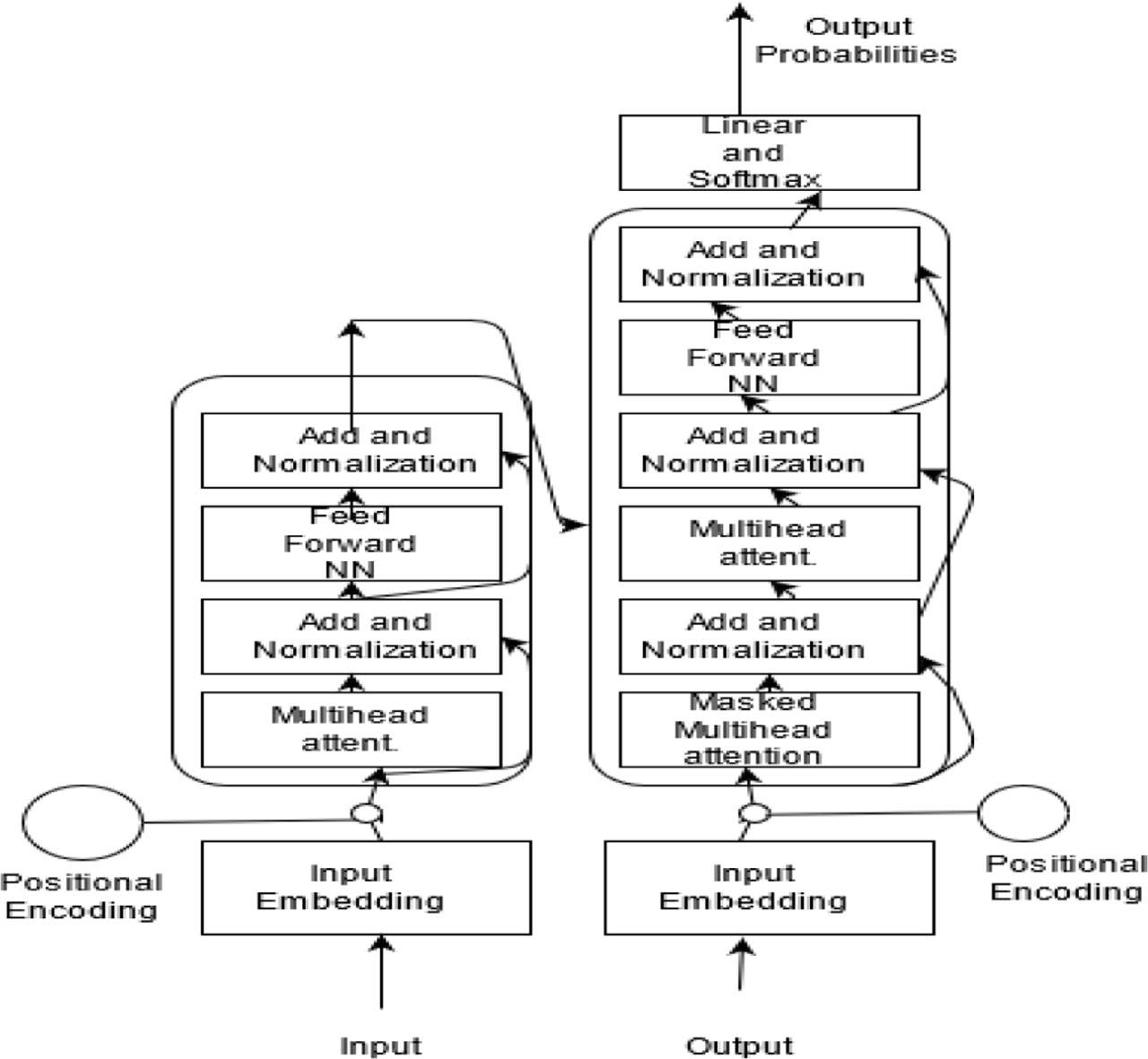
Figure 6:
Transformer model.
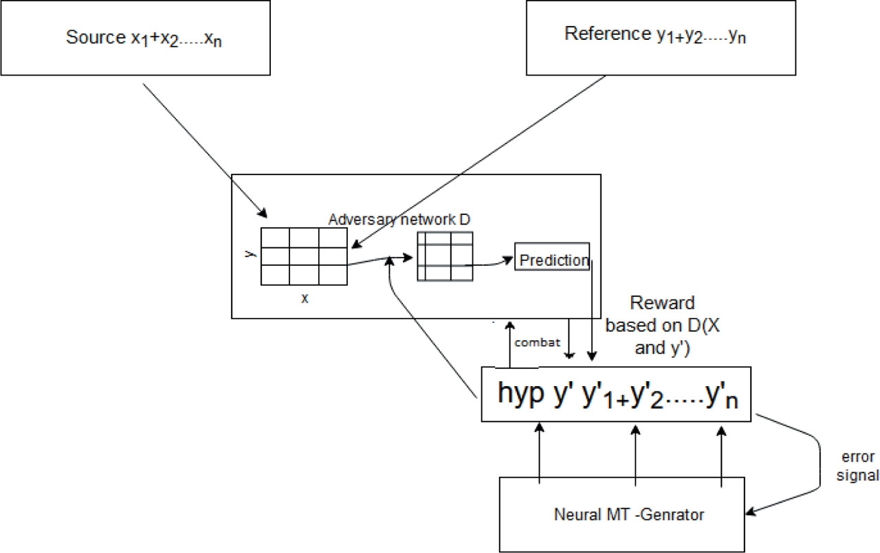
Figure 7:
The generative adversarial network (GAN) model in the NMT case.
Table 1.
Generic hyper-parameters in NMT-based model.
| Model | Type of MT | Hyper-parameters |
|---|---|---|
| Deep learning models | NMT | Hidden layers, learning rate, activation function, epochs, batch size, dropout, regularization |
Table 2.
WMT-14 English–French test results showed that 60L-12L ADMIN outperforms the default base model 6L-6L in different automatic metrics (Liu et al. [35]).
| Model | Param | TER | METEOR | BLEU |
|---|---|---|---|---|
| 6L-6L Default | 67M | 42.2 | 60.5 | 41.3 |
| 6L-6L ADMIN | 67M | 41.8 | 60.7 | 41.5 |
| 60L-12LDefault | 262M | Diverge | Diverge | Diverge |
| 60L-12LADMIN | 262M | 40.3 | 62.4 | 43.8 |
Table 3.
WMT-14 English–German test results show that ADMIN outperforms the default base model 6L-6L in different automatic metrics (Liu et al. [35]).
| Model | Param | TER | METEOR | BLEU |
|---|---|---|---|---|
| 6L-6L Default | 61M | 54.4 | 46.6 | 27.6 |
| 6L-6L ADMIN | 61M | 54.1 | 46.7 | 27.7 |
| 60L-12LDefault | 256M | Diverge | Diverge | Diverge |
| 60L-12LADMIN | 256M | 51.8 | 48.3 | 30.1 |
Table 4.
Models per data set and their best BLEU scores and respective hyper-parameter configurations (Zhang and Duh [36]).
| Data set | No. of models | Best BLEU | BPE | No. of layers | No. of embedding | No. of hidden layers | No. of attention heads | Init-lr |
|---|---|---|---|---|---|---|---|---|
| Chinese–English | 118 | 14.66 | 30k | 4 | 512 | 1024 | 16 | 3e-4 |
| Russian–English | 176 | 20.23 | 10k | 4 | 256 | 2048 | 8 | 3e-4 |
| Japanese–English | 150 | 16.41 | 30k | 4 | 512 | 2048 | 8 | 3e-4 |
| English–Japanese | 168 | 20.74 | 10k | 4 | 1024 | 2048 | 8 | 3e-4 |
| Swahili–English | 767 | 26.09 | 1k | 2 | 256 | 1024 | 8 | 6e-4 |
| Somali–English | 604 | 11.23 | 8k | 2 | 512 | 1024 | 8 | 3e-4 |
Table 5.
MT models for different language pairs in a GPU-based single-node and multiple-node environment with a wider range of hyper-parameters and their BLEU scores (Lim et al. [11]).
| Cell | Learning rate | ro→en P100 | ro→en V100 | en→ro P100 | en→ro V100 | de→en P100 | de→en V100 | en→de P100 | en→de V100 |
|---|---|---|---|---|---|---|---|---|---|
| GRU | le-3 | 35.53 | 35.43 | 19.19 | 19.28 | 28.00 | 27.84 | 20.43 | 20.61 |
| 5e-3 | 34.37 | 34.05 | 19.07 | 19.16 | 26.05 | 22.16 | N/A | 19.01 | |
| le-4 | 35.47 | 35.46 | 19.45 | 19.49 | 27.37 | 27.81 | Dnf | 21.41 | |
| LSTM | le-3 | 34.27 | 35.61 | 19.29 | 19.64 | 28.62 | 28.83 | 21.70 | 21.69 |
| 5e-3 | 35.05 | 34.99 | 19.48 | 19.43 | N/A | 24.36 | 18.53 | 18.01 | |
| le-4 | 35.41 | 35.28 | 19.43 | 19.48 | N/A | 28.50 | Dnf | Dnf | |
| GRU | le-3 | 34.22 | 34.17 | 19.42 | 19.43 | 33.03 | 32.55 | 26.55 | 26.85 |
| 5e-3 | 33.13 | 32.74 | 19.31 | 18.97 | 31.04 | 26.76 | N/A | 26.02 | |
| le-4 | 33.67 | 34.44 | 18.98 | 19.69 | 33.15 | 33.12 | Dnf | 28.43 | |
| LSTM | le-3 | 33.10 | 33.95 | 19.56 | 19.08 | 33.10 | 33.89 | 28.79 | 28.84 |
| 5e-3 | 33.10 | 33.52 | 19.13 | 19.51 | N/A | 29.16 | 24.12 | 24.12 | |
| le-4 | 33.29 | 32.92 | 19.14 | 19.23 | N/A | 33.44 | Dnf | Dnf |
Table 6.
NMT models with some other range of learning rate (hyper-parameter) (Lim et al. [11]).
| Cell | Learning rate | ro→en P100 | ro→en t | ro→en V100 | ro→en t | de→en P100 | de→en t | de→en V100 | de→en t |
|---|---|---|---|---|---|---|---|---|---|
| GRU | 0.0 | 34.47 | 6:29 | 34.47 | 4:43 | 32.29 | 9:48 | 31.61 | 6:15 |
| 0.2 | 35.53 | 8:48 | 35.43 | 6:21 | 33.03 | 18:47 | 32.55 | 19:40 | |
| 0.3 | 35.36 | 12:21 | 35.15 | 7:28 | 31.36 | 10:14 | 31.50 | 9:33 | |
| 0.5 | 34.50 | 12:20 | 34.67 | 17:18 | 29.64 | 11:09 | 30.21 | 11.09 | |
| LSTM | 0.0 | 34.84 | 6:29 | 34.65 | 4:46 | 32.84 | 12:17 | 32.88 | 7:37 |
| 0.2 | 34.27 | 8:10 | 35.61 | 6:34 | 33.10 | 16:33 | 33.89 | 13:39 | |
| 0.3 | 35.67 | 9:56 | 35.37 | 11:29 | 33.45 | 20.02 | 33.51 | 15:51 | |
| 0.5 | 34.50 | 15:13 | 34.33 | 12:45 | 32.67 | 20.02 | 32.20 | 13.03 |
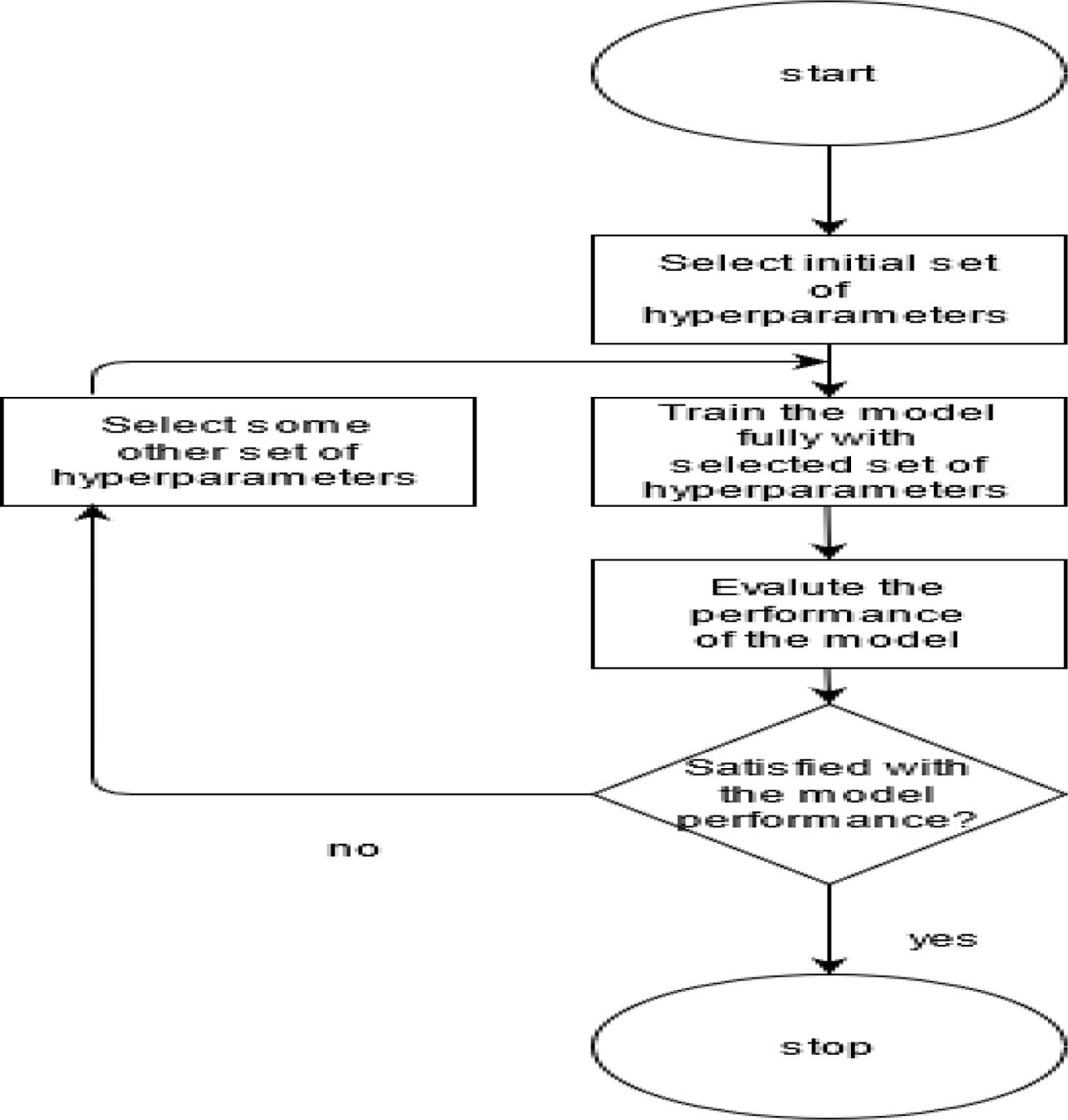
Figure 8:
Typical machine learning model building steps.
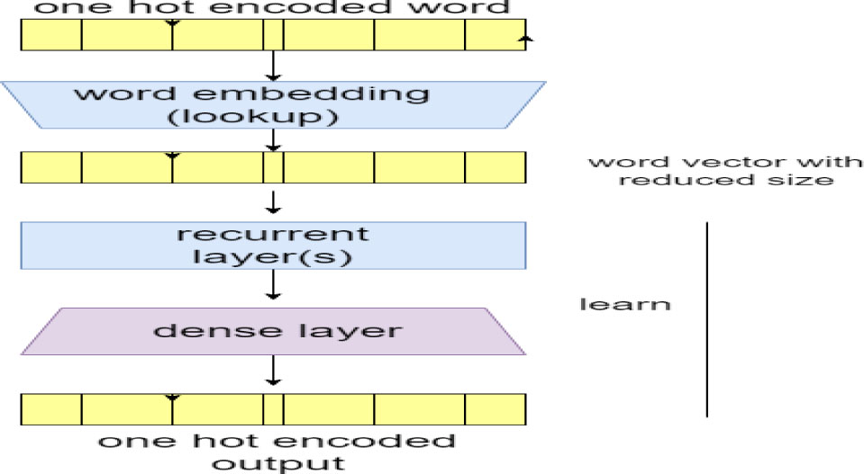
Figure 9:
Schematic representation of the NMT model.
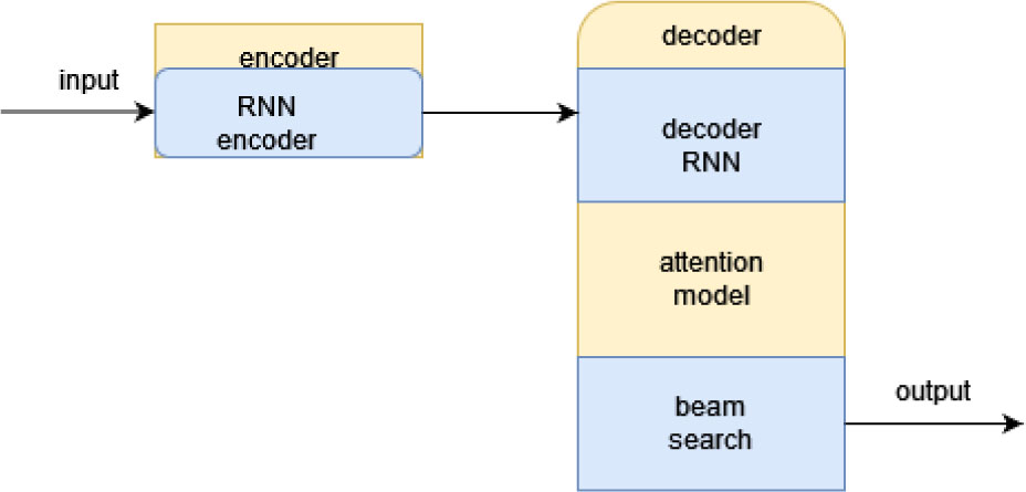
Figure 10:
Encoder–decoder-based NMT model.
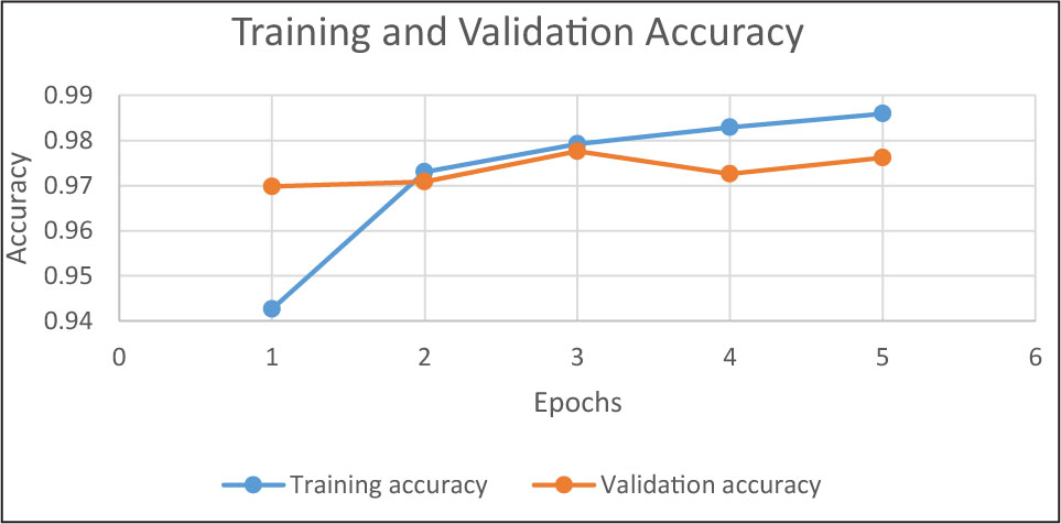
Figure 11:
Training and validation accuracy with five epochs.
Table 7.
Training and validation accuracy of our model with five epochs.
| Epochs | Training accuracy | Validation accuracy |
|---|---|---|
| 1 | 0.9426 | 0.9698 |
| 2 | 0.9730 | 0.9708 |
| 3 | 0.9792 | 0.9776 |
| 4 | 0.9829 | 0.9726 |
| 5 | 0.9859 | 0.9762 |
Table 8.
Training and validation accuracy of our model with a higher number of epochs.
| Epochs | Training accuracy | Validation accuracy |
|---|---|---|
| 1 | 0.9431 | 0.9606 |
| 2 | 0.9742 | 0.9729 |
| 3 | 0.9796 | 0.9777 |
| 4 | 0.9835 | 0.9748 |
| 5 | 0.9865 | 0.9794 |
| 6 | 0.9872 | 0.9802 |
| 7 | 0.9896 | 0.9830 |
| 8 | 0.9898 | 0.9782 |
| 9 | 0.9916 | 0.9764 |
| 10 | 0.9924 | 0.9799 |
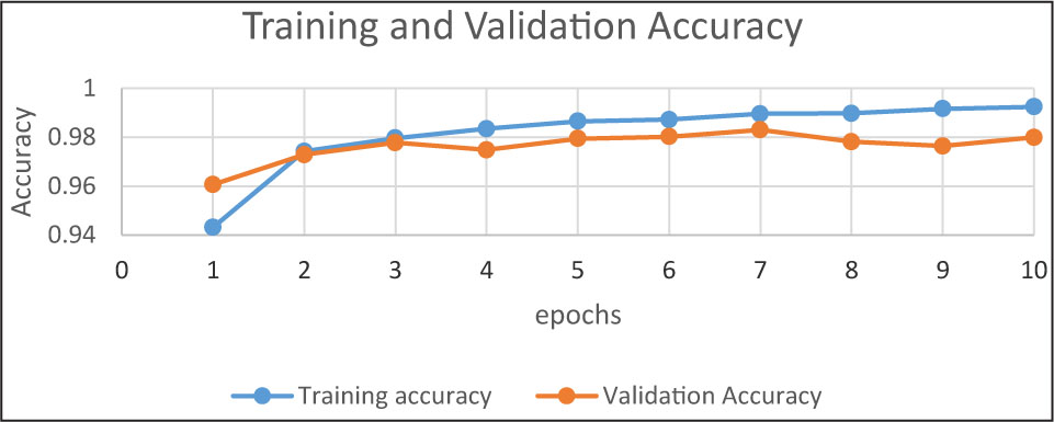
Figure 12:
There is a slight improvement in training and validation accuracy with increasing the number of epochs up to 10.
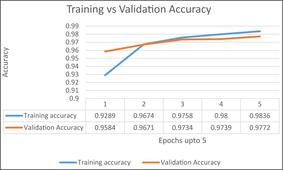
Figure 13:
Graphical representation of training and validation accuracy with reduced units in different layers and up to five epochs.
Table 9.
Training and validation accuracy with 100 units in different layers with five epochs.
| Epochs | Training accuracy | Validation accuracy |
|---|---|---|
| 1 | 0.9289 | 0.9584 |
| 2 | 0.9674 | 0.9671 |
| 3 | 0.9758 | 0.9734 |
| 4 | 0.9800 | 0.9739 |
| 5 | 0.9836 | 0.9772 |
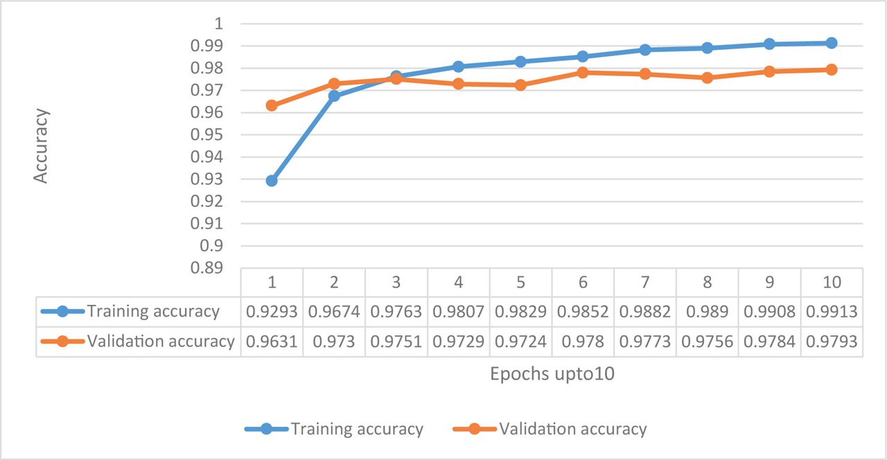
Figure 14:
Graphical representation of training and validation accuracy with reduced units per layer and increased number of epochs, i.e., up to 10.
Table 10.
Training and validation accuracy with 100 units in different layers with 10 epochs.
| Epochs | Training accuracy | Validation accuracy |
|---|---|---|
| 1 | 0.9293 | 0.9631 |
| 2 | 0.9674 | 0.9730 |
| 3 | 0.9763 | 0.9751 |
| 4 | 0.9807 | 0.9729 |
| 5 | 0.9829 | 0.9724 |
| 6 | 0.9852 | 0.9780 |
| 7 | 0.9882 | 0.9773 |
| 8 | 0.9890 | 0.9756 |
| 9 | 0.9908 | 0.9784 |
| 10 | 0.9913 | 0.9793 |

Figure 15:
Snapshots of the English–Bangla parallel corpus collected from TDIL.
Table 11.
Statistics of English to Bangla tourism corpus (text) collected from TDIL.
| Corpus (English to Bangla) | Size in terms of sentence pairs |
|---|---|
| Tourism | 11,976 |
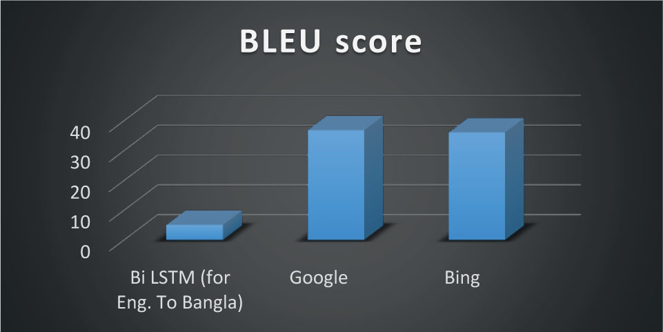
Figure 16:
BLEU scores produced by different NMT models for the first test data.
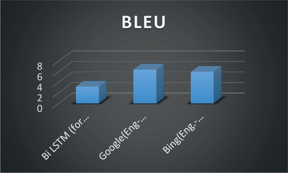
Figure 17:
BLEU scores generated by different NMT models for the second test data.
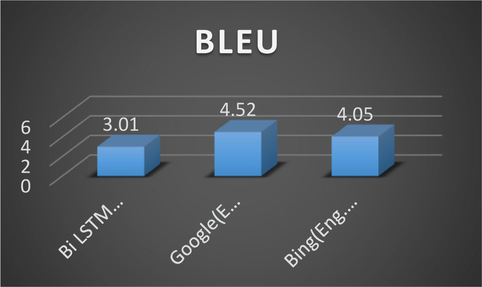
Figure 18:
BLEU score produced by various NMT models on third test data.
Table 12.
Performance of BiLSTM, Google Translate, and Bing in terms of the automatic metric BLEU.
| Model | Hyper-parameter | BLEU score |
|---|---|---|
| BiLSTM (for English to Bangla; 1st sentence) | Optimizer = Adam; | 4.1 |
| BiLSTM (for English to Bangla; 2nd sentence) | Learning rate = 0.001; | 3.2 |
| BiLSTM (for English to Bangla; 3rd sentence) | No. of encoder and decoder layers = 6 | 3.01 |
Table 13.
Translations generated by Google and Bing.
| Translators | Language pair | BLEU |
|---|---|---|
| English ⇒ Bangla (1st sentence) | 36.84 | |
| English ⇒ Bangla (2nd sentence) | 6.42 | |
| English ⇒ Bangla (3rd sentence) | 4.52 | |
| Bing | English ⇒ Bangla (1st sentence) | 36.11 |
| English ⇒ Bangla (2nd sentence) | 6.01 | |
| English ⇒ Bangla (3rd sentence) | 4.05 |