
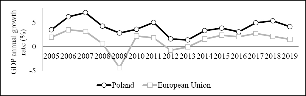
Figure 1.
Poland’s and EU’s GDP annual growth rate (%) 2005–2019. Source: Own work based on data from the World Bank [2020].
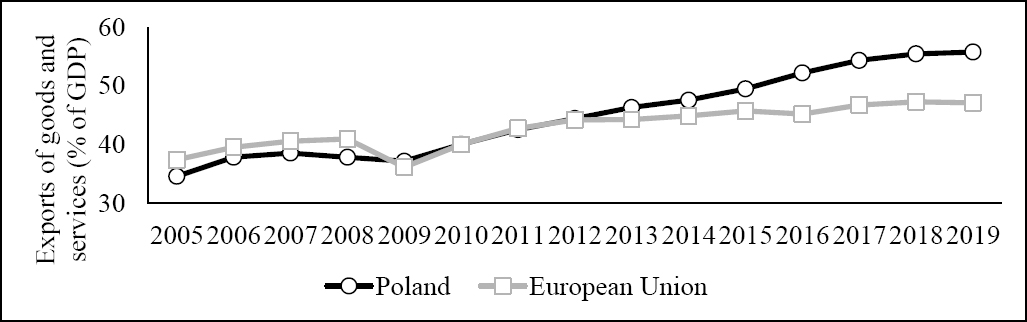
Figure 2.
Poland’s and EU’s exports of goods and services (% of GDP) 2005–2019. Source: Own work based on data from the World Bank [2020].
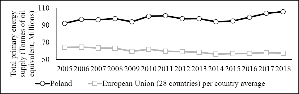
Figure 3.
Poland’s and EU’s total primary energy supply (tons of oil equivalent, millions) 2005–2018. Source: Own work based on data from the OECD [2020].
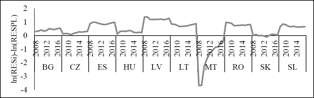
Figure 4.
Relative share of renewable energy in gross final energy consumption 2005–2018. BG, Bulgaria; CZ, Czechia; ES, Estonia; HU, Hungary; LT, Lithuania; LV, Latvia; MT, Malta; RO, Romania; SK, Slovakia; SL, Slovenia. Source: Own work based on data from the Eurostat [2020c].
Table 1.
Variables description
| Group | Description (source) | Formula |
|---|---|---|
| Dependent variable | Relative RCA* | |
| Heckscher–Ohlin theory | Relative physical capital per worker endowment | |
| Relative human capital endowment | ||
| Ricardian theory | Relative labor productivity | |
| Energy variables | Total primary energy supply [OECD, 2020] | ln (TPESi) – ln (TPESPL) |
| Energy import dependency [Eurostat, 2020b] | ln (EIDi)–ln(EIDPL) | |
| Share of renewable energy in gross final energy consumption [Eurostat, 2020c] | ln (RESi)–ln(RESPL) | |
| Energy intensity [Eurostat, 2020d] | ln(EIi)–ln(EiPL) | |
| Greenhouse gas emissions [Eurostat, 2020e] | ln (GHGi)–ln (GHGPL) |
Table 2.
Values of VIFs
| Variable | ln(TPESi) – ln(TPESPL) | ln(RESi) – ln(RESPL) | ln(GHGi) – ln(GHGPL) | ln(EIi) – ln(EiPL) | ln(EIDi) – ln(EIDPL) | Mean VIF | |||
| VIF | 10.480 | 5.540 | 3.930 | 3.370 | 2.980 | 2.760 | 2.590 | 2.490 | 4.270 |
1 Source: Own calculations with STATA 15 based on data from the World Bank [2020], OECD [2020], University of Groningen [2019a], and Eurostat [2020a-e].
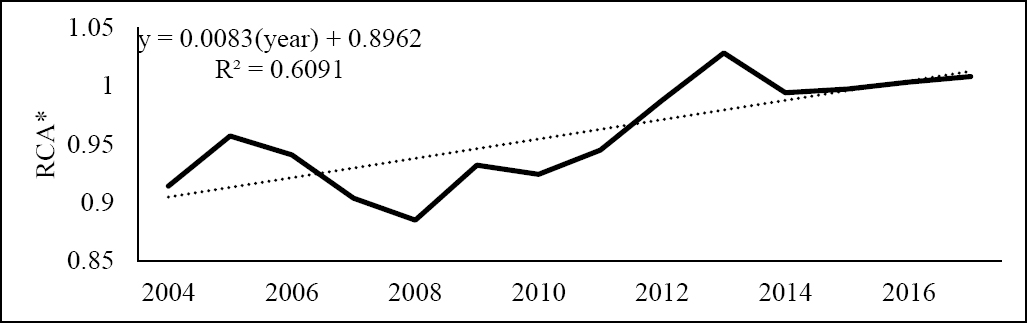
Figure 5.
Poland’s RCA* 2004–2017.
Source: Own work based on data from the World Bank [2020].
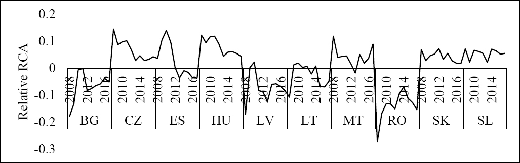
Figure 6.
Relative RCA* for the analyzed economies. BG, Bulgaria; CZ, Czechia; ES, Estonia; HU, Hungary; LT, Lithuania; LV, Latvia; MT, Malta; RO, Romania; SK, Slovakia; SL, Slovenia.
Source: Own work based on data from the World Bank [2020].
Table 3.
Results of econometric modeling
| Model 1 (Eq. [3]) | Model 2 (Eq. [4]) | Model 3 (Eq. [5]) | ||||
|---|---|---|---|---|---|---|
| Coef. | P > t | Coef. | P > t | Coef. | P > t | |
| ln(TPESi) – ln(TPESPL) | –0.220* | 0.058 | –0.213** | 0.023 | –0.170* | 0.078 |
| ln(EIDi) – ln(EIDPL) | –0.013 | 0.743 | - | - | - | - |
| ln(RES) – ln(RESPL) | –0.018** | 0.047 | –0.020** | 0.018 | - | - |
| ln(EIi) – ln(EIPL) | –0.031 | 0.671 | - | - | - | - |
| ln(GHGi) – ln(GHGPL) | 0.021 | 0.684 | - | - | - | - |
| 195.925* | 0.094 | 191.537 | 0.105 | 212.377* | 0.068 | |
| 1.482** | 0.015 | 1.519** | 0.015 | 1.533** | 0.016 | |
| –0.058 | 0.680 | –0.045 | 0.760 | –0.057 | 0.700 | |
| β0 | –0.600 | 0.021 | –0.595 | 0.006 | –0.515 | 0.026 |
| Lagram–Multiplier | 0.001 | 0.001 | 0.001 | |||
| Modified Wald | 0.000 | 0.000 | 0.000 | |||
| Jarque–Bera P-value | 0.016 | 0.021 | 0.126 | |||
| Shapiro–Wilk P-value | 0.000 | 0.000 | 0.017 | |||
| Levin–Lin–Chu P-value | 0.000 | 0.000 | 0.000 | |||
| Harris–Tzavalis P-value | 0.000 | 0.000 | 0.000 | |||
| R2 within | 0.263 | 0.259 | 0.235 | |||
| R2 between | 0.235 | 0.239 | 0.277 | |||
| R2 overall | 0.193 | 0.196 | 0.228 | |||
| Prob. > F | 0.000 | 0.001 | 0.001 | |||
1 Note: ** and * denote significance at the 5% and 10% levels, respectively.
Source: Own calculations with STATA 15 based on data from the World Bank [2020], OECD [2020], University of Groningen [2019a], and Eurostat [2020a-e].