
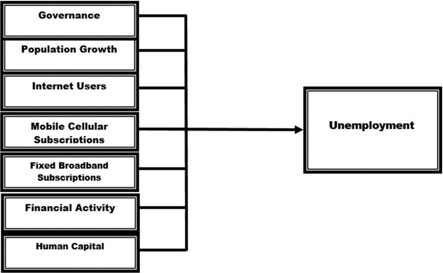
Figure 1
Conceptual framework.
Table 1
Variable description and sources
| Variable | Description | Units | Source |
|---|---|---|---|
| UE | Unemployment rate | % of the total labor force | World Bank |
| GOV | Governance | Index | Worldwide Governance Indicators |
| POP | Population growth | Annual % | World Bank |
| IU | Internet users | Per 100 people | World Bank |
| MCS | Mobile cellular subscriptions | Per 100 people | World Bank |
| FBS | Fixed broadband subscriptions | Per 100 people | World Bank |
| FA | Financial activity | Credit | FDSD |
| HC | Human capital (education) | Gross % of enrollment | World Bank |
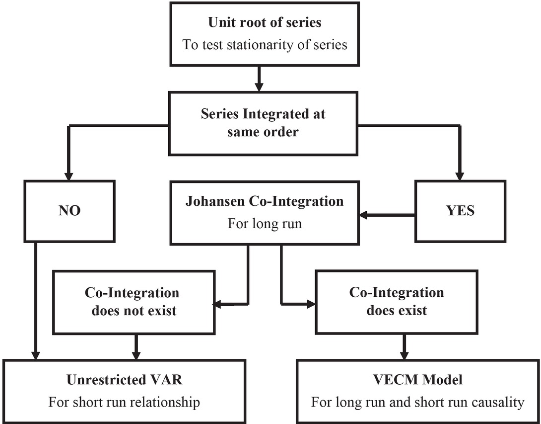
Figure 2
Methodology flow chart.
Table 2
Descriptive statistics
| UE | GOV | POP | IU | MBS | FBS | HC | FA | |
|---|---|---|---|---|---|---|---|---|
| Mean | 4.4891 | 0.0045 | −0.0259 | −0.0798 | 26.04072 | 1.0522 | −0.0061 | 40.194 |
| Median | 3.9120 | 0.0074 | −0.0357 | 0.3329 | 4.761983 | 0.4996 | −0.0966 | 44.160 |
| Maximum | 13.030 | 0.5988 | 0.9557 | 9.5000 | 115.3790 | 5.7863 | 2.7491 | 86.186 |
| Minimum | 0.6500 | −0.8829 | −1.0564 | −21.824 | 0.000000 | −2.1401 | −3.4107 | −13.850 |
| SD | 2.7037 | 0.2420 | 0.2114 | 3.7815 | 32.52466 | 1.6768 | 1.4838 | 23.982 |
| Skewness | 1.2746 | −0.4964 | 0.2574 | −2.5320 | 0.884126 | 1.1617 | −0.2005 | −0.6672 |
| Kurtosis | 4.1690 | 4.1290 | 15.782 | 13.930 | 2.372628 | 4.0800 | 2.2792 | 2.7402 |
| Jarque–Bera | 46.539 | 13.373 | 968.27 | 858.61 | 20.79126 | 38.842 | 4.0249 | 10.936 |
| Probability | 0.0000 | 0.0012 | 0.0000 | 0.0000 | 0.0000 | 0.0000 | 0.1336 | 0.004219 |
| Observations | 161 | 161 | 161 | 161 | 161 | 161 | 161 | 161 |
[i] SD, standard deviation.
Table 3
Panel unit root test
| Levin, Lin & Chu test | Im, Pesaran and Shin test | ||||||||
|---|---|---|---|---|---|---|---|---|---|
| Variables | Level | First difference | Level | First Difference | Decision | ||||
| T−statistics | P−value | T−statistics | P−value | T−statistics | P−value | T−statistics | P−value | ||
| UE | −2.427 | 0.007 | −9.034 | 0.00 | −0.454 | 0.324 | −9.715 | 0.00 | I(1) |
| GOV | −1.626 | 0.051 | −8.769 | 0.00 | −1.28 | 0.098 | −10.05 | 0.00 | I(1) |
| POP | 1.346 | 0.910 | −3.234 | 0.00 | −2.34 | 0.009 | −7.624 | 0.00 | I(1) |
| IU | 5.966 | 1.000 | −9.196 | 0.00 | −1.41 | 0.078 | −9.829 | 0.00 | I(1) |
| MCS | −1.538 | 0.062 | −5.641 | 0.00 | −3.38 | 0.000 | 49.68 | 0.00 | I(1) |
| FBS | 0.114 | 0.545 | −4.275 | 0.00 | −0.832 | 0.202 | 49.17 | 0.00 | I(1) |
| FA | −0.306 | 0.379 | −10.21 | 0.00 | 0.007 | 0.503 | −7.058 | 0.00 | I(1) |
| HC | 0.333 | 0.630 | −8.735 | 0.00 | 1.400 | 0.919 | −5.99 | 0.00 | I(1) |
[i] Null hypothesis: There is a unit root/variable is not stationary.
Table 4
Optimal lag length selection
| Lag | Log (L) | LR | FPE | AIC | SC | HQ |
|---|---|---|---|---|---|---|
| 0 | −1785.819 | NA | 20168.37 | 32.61488 | 32.81128 | 32.69454 |
| 1 | −1085.927 | 1285.255 | 0.192653 | 21.05322 | 22.82081 | 21.77016 |
| 2 | −939.9511 | 246.8322 | 0.044144 | 19.56275 | 22.90152 | 20.91697 |
| 3 | −897.7784 | 65.17604 | 0.068647 | 19.95961 | 24.86957 | 21.95112 |
| 4 | −841.4533 | 78.85510 | 0.086160 | 20.09915 | 26.58030 | 22.72794 |
Table 5
Results for Johansen cointegration test
| Hypothesized no. of CE(s) | Fisher’s statistic* (from trace test) | p | Fisher’s statistic* (from max-Eigen test) | p |
|---|---|---|---|---|
| None | 6.931 | 0.7319 | 6.931 | 0.7319 |
| At most 1 | 5.545 | 0.8519 | 23.97 | 0.0077* |
| At most 2 | 1.386 | 0.9992 | 75.07 | 0.0000* |
| At most 3 | 92.10 | 0.0000* | 92.10 | 0.0000* |
| At most 4 | 205.2 | 0.0000* | 124.7 | 0.0000* |
| At most 5 | 117.9 | 0.0000* | 84.62 | 0.0000* |
| At most 6 | 55.01 | 0.0000* | 41.14 | 0.0000* |
| At most 7 | 35.30 | 0.0001* | 35.30 | 0.0001* |
[i] Null hypothesis: There is no cointegration.
CE, cointegration equation.
*Cointegration exits in this equation.
Table 6
Results for Kao Residual Cointegration Test
| Kao Residual Cointegration Test | t-Statistic | p |
|---|---|---|
| ADF | −5.252339 | 0.0000 |
| Residual variance | 29.53757 | |
| HAC variance | 27.06740 |
[i] Null hypothesis: There is no cointegration.
Table 7
Long-run relationship of VECM
| Variables | Coefficients | Standard errors | t−value |
|---|---|---|---|
| FA (–1) | +0.620559 | 0.95581 | −3.59327 |
| FBS (–1) | −0.531762 | 15.2189 | 2.64497 |
| GOV (–1) | −0.526023 | 91.4792 | 3.20063 |
| HC (–1) | −0.450647 | 9.79514 | 2.60362 |
| IU (–1) | −0.334496 | 7.54714 | 4.85044 |
| MCS (–1) | −0.127821 | 0.68663 | 2.48479 |
| POP (–1) | +0.802420 | 193.675 | −8.16830 |
| C | 10.84378 | ||
| CointEq1 | −0.072136 | 0.01545 | −4.66826 |
| R-squared | 0.641065 | ||
| F-statistic | 2.535735 |
[i] VECM, vector error correction model.
Table 8
Results of the Granger causality test
| Granger causality test: emerging and growth leading economies | |||
|---|---|---|---|
| Null hypothesis | F-statistics | p | Decision |
| GOV does not Granger cause UE | 3.04895 | 0.0505** | Bidirectional |
| UE does not Granger cause GOV | 2.90152 | 0.0582** | Causality |
| POP does not Granger cause UE | 1.05352 | 0.3514 | No |
| UE does not Granger cause POP | 1.62622 | 0.2003 | Causality |
| HC does not Granger cause UE | 0.85811 | 0.4265 | No |
| UE does not Granger cause HC | 0.45764 | 0.6339 | Causality |
| IU does not Granger cause UE | 2.82781 | 0.0947** | Unidirectional |
| UE does not Granger cause IU | 1.27496 | 0.2606 | Causality |
| MCS does not Granger cause UE | 0.26316 | 0.7690 | No |
| UE does not Granger cause MCS | 0.27047 | 0.7634 | Causality |
| FBS does not Granger cause UE | 0.55304 | 0.4582 | Unidirectional |
| UE does not Granger cause FBS | 6.51372 | 0.0117* | Causality |
| FA does not Granger cause UE | 0.76037 | 0.4696 | No |
| UE does not Granger cause FA | 0.80089 | 0.4512 | Causality |
[i] Decision rule: Reject H0, if the p-value is less than 0.05.
*Signifies the refusal of a null hypothesis at the 5% level of significance.
**Signifies the refusal of a null hypothesis at the 10% level of significance.
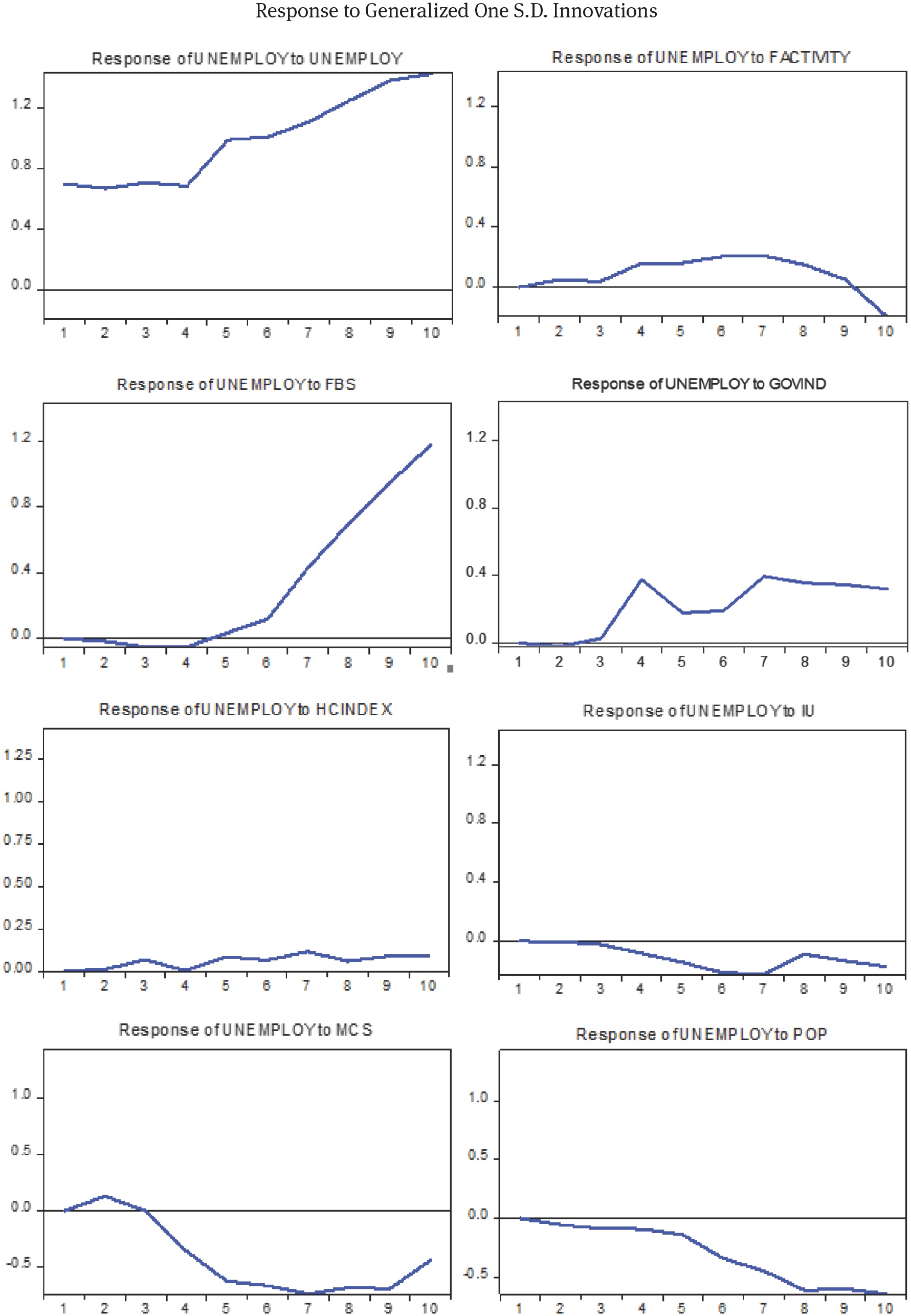
Figure 3
Impulse Response Function: Response to Generalized 1 SD Innovations. SD, standard deviation.
Table 9
Results for forecast error variance decompositions
| Period | SE | UE | GOV | POP | IU | MCS | FBS | FA | HC |
|---|---|---|---|---|---|---|---|---|---|
| 1 | 0.700 | 100.0 | 0.000 | 0.000 | 0.000 | 0.000 | 0.000 | 0.000 | 0.000 |
| 2 | 0.981 | 97.54 | 0.256 | 0.026 | 0.038 | 0.013 | 0.000 | 1.816 | 0.307 |
| 3 | 1.217 | 97.24 | 0.261 | 0.198 | 0.068 | 0.312 | 0.032 | 1.182 | 0.699 |
| 4 | 1.504 | 84.46 | 1.274 | 0.254 | 6.263 | 0.204 | 0.316 | 6.398 | 0.825 |
| 5 | 1.934 | 77.34 | 1.461 | 0.184 | 4.640 | 0.313 | 0.734 | 14.294 | 1.027 |
| 6 | 2.337 | 71.70 | 1.763 | 0.387 | 3.840 | 0.291 | 1.342 | 17.824 | 2.843 |
| 7 | 2.809 | 65.31 | 1.772 | 2.655 | 4.638 | 0.372 | 1.564 | 19.187 | 4.492 |
| 8 | 3.310 | 61.43 | 1.482 | 6.417 | 4.493 | 0.300 | 1.196 | 18.027 | 6.644 |
| 9 | 3.841 | 58.62 | 1.117 | 10.85 | 4.144 | 0.277 | 1.009 | 16.616 | 7.356 |
| 10 | 4.354 | 56.41 | 1.058 | 15.73 | 3.763 | 0.259 | 0.939 | 13.943 | 7.888 |
Table 10
Serial Correlation Test
| Lags | LM-Stat | p |
|---|---|---|
| 1 | 98.19758 | 0.0039 |
| 2 | 104.3011 | 0.0011 |
| 3 | 95.75344 | 0.0062 |
| 4 | 79.53887 | 0.0912 |
| 5 | 83.15507 | 0.0541 |
[i] Null hypothesis: There is no serial correlation.
Table 11
Heteroscedasticity Test (Breusch–Pagan–Godfrey)
| Test | Chi-square | p |
|---|---|---|
| Joint test | 3067.172 | 0.0683 |
[i] Null hypothesis: homoscedasticity.
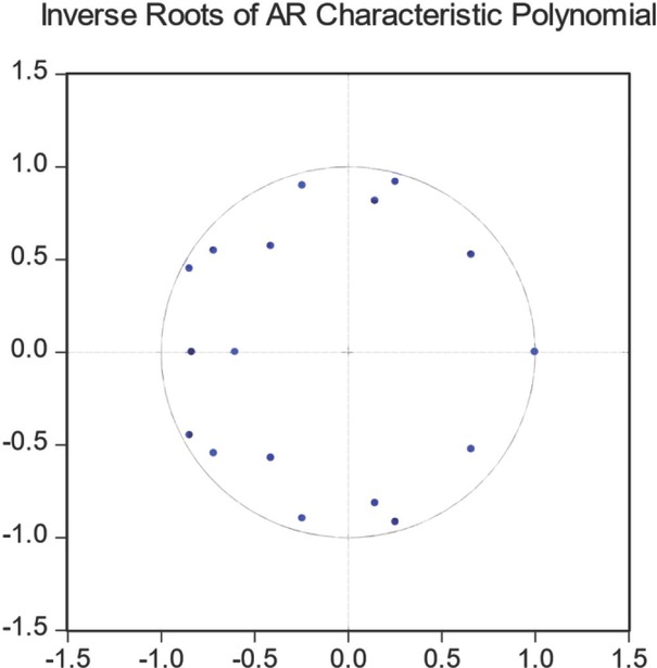
Figure 4
Model stability test.
Table 12
Multicollinearity Test
| Variables | FA | FBS | GOV | HC | IU | MBS | POP |
|---|---|---|---|---|---|---|---|
| FA | 1.00 | ||||||
| – | |||||||
| FBS | −0.56 | 1.00 | |||||
| −8.16 | – | ||||||
| GOV | −0.10 | 0.16 | 1.00 | ||||
| −1.20 | 2.00 | – | |||||
| HC | 0.65 | −0.23 | −0.04 | 1.00 | |||
| 10.3 | −2.85 | −0.51 | – | ||||
| IU | 0.26 | −0.08 | −0.14 | 0.21 | 1.00 | ||
| 3.22 | −1.03 | −1.77 | 2.58 | – | |||
| MBS | −0.36 | 0.13 | 0.17 | −0.21 | −0.27 | 1.00 | |
| −4.70 | 1.58 | 2.08 | −2.54 | −3.38 | – | ||
| POP | −0.08 | 0.15 | 0.06 | −0.10 | −0.00 | 0.04 | 1.00 |
| −1.01 | 1.83 | 0.72 | −1.26 | −0.10 | 0.53 | – | |
| UE | −0.24 | 0.04 | 0.02 | −0.03 | 0.09 | −0.23 | −0.28 |
| −2.99 | 0.57 | 0.34 | −0.47 | 1.08 | −2.82 | −3.46 |
Table 13
Lags exclusion Wald test
| Chi-squared test statistics for lag exclusion | |||||||||
|---|---|---|---|---|---|---|---|---|---|
| d(UE) | d(FA) | d(FBS) | d(GOV) | d(HC) | d(IU) | d(MCS) | d(POP) | Joint | |
| DLag 1 | 2.506 | 14.929 | 17.171 | 27.848 | 16.686 | 10.531 | 30.875 | 105.051 | 287.87 |
| [0.9614] | [0.0605] | [0.0284] | [0.0005] | [0.0335] | [0.229] | [0.0001] | [0.0000] | [0.000] | |
| DLag 2 | 3.002 | 19.338 | 31.285 | 12.528 | 21.656 | 8.153 | 13.469 | 26.211 | 154.698 |
| [0.9342] | [0.0132] | [0.0001] | [0.129] | [0.0056] | [0.418] | [0.0967] | [0.0010] | [0.000] | |
| DLag 3 | 11.082 | 15.685 | 12.816 | 2.6085 | 19.692 | 2.411 | 4.8671 | 35.783 | 110.890 |
| [0.1971] | [0.0471] | [0.1183] | [0.956] | [0.0116] | [0.965] | [0.7717] | [0.0000] | [0.0003] | |
| DLag 4 | 14.027 | 16.400 | 76.592 | 3.212 | 13.160 | 13 .564 | 19.335 | 47.179 | 200.654 |
| [0.0011] | [0.0370] | [0.0000] | [0.9203] | [0.1065] | [0.093] | [0.0132] | [0.0000] | [0.0000] | |
| df | 8 | 8 | 8 | 8 | 8 | 8 | 8 | 8 | 64 |
[i] The numbers written in [] are p-values.