
1. Introduction
Fractional calculus has been developed by many scientists from the past to the present and various fractional integral and derivative operators have been defined, see Baleanu et al. [1], Hilfer [2], Miller and Ross [3], Samko et al. [4], Podlubny [5] and Kilbas et al. [6]. Later, scientists were interested in fractional order differential equations and obtained their solutions by integral transformations, see Tanriverdi et al. [7], Ata and Kıymaz [8], Luchko et al. [9], Ata and Kıymaz [10] and Lin and Lu [11].
Special functions have an important role in many scientific fields such as physics, mathematics and engineering. Some of these special functions are gamma, beta, Gauss hypergeometric and confluent hypergeometric functions and we give these special functions below.
The gamma function Andrews et al. [12] for ℜ(σ) > 0 is defined by
The beta function Andrews et al. [12] for ℜ(σ) > 0 and ℜ(τ) > 0 is given by
The Gauss hypergeometric function Kilbas et al. [6] for ℜ(ϑ3) > ℜ(ϑ2) > 0 is defined by
The confluent hypergeometric function Kilbas et al. [6] for ℜ(ϑ3) > ℜ(ϑ2) > 0 is given by
Here denotes (·)k is known as the Pochhammer symbol Andrews et al. [12] and defined by
Scientists have obtained various generalizations of these special functions by working on the special functions mentioned above. We let ℜ(p) > 0, ℜ(q) > 0, ℜ(κ) > 0, ℜ(μ) > 0, ℜ(α) > 0, ℜ(β) > 0, ℜ(σ) > 0, ℜ(τ) > 0, ℜ(ϑ3) > ℜ(ϑ2) > 0 unless otherwise stated.
The generalized gamma functions were introduced by Parmar [13] and Şahin et al. [14] respectively as follows
The generalized beta functions were introduced by Khan and Husain [15], Çetinkaya et al. [16] and Şahin et al. [14] respectively as follows
The generalized Gauss and confluent hypergeometric functions were introduced by Khan and Husain [15] and Şahin et al. [14] respectively as follows
andAlso for other studies that can be found in the specific literature, see Abubakar [17], Abubakar [18], Al-Gonah and Mohammed [19], Ata and Kıymaz [20], Ata [21], Ata and Kıymaz [22], Atash et al. [23], Chaudhry and Zubair [24], Chaudhry et al. [25], Chaudhry et al. [26], Choi et al. [27], Goswami et al. [28], Goyal et al. [29], Kulip et al. [30], Lee et al. [31], Mubeen et al. [32], Özergin et al. [33], Rahman et al. [34], Rahman et al. [35], Shadab et al. [36], Ata and Kıymaz [37], Srivastava et al. [38], Ata [39], Kıymaz et al. [40], Srivastava et al. [41] and Kıymaz et al. [42].
The motivation of this paper is to introduce special functions with general kernel that generate generalized gamma, beta, Gauss hypergeometric and confluent hypergeometric functions and to obtain solutions of fractional partial differential equations involving special functions with general kernel.
The remainder of this paper is organized as follows: In Section 2, we provide the basic information needed throughout the paper. In Section 3, we describe the special functions with general kernel and show that they generate other special functions. In Section 4, we give some properties of the special functions with general kernel. In Section 5, we obtain solutions of fractional partial differential equations involving special functions with general kernel and then we present graphs for some specific values. In Section 6, we give the beta distribution with general kernel and introduce the incomplete beta function with general kernel. Finally, we give conclusions and remarks in Section 7.
2. Preliminaries
The Laplace and inverse Laplace transforms are obtained from the Fourier integral formula in Debnath and Bhatta [43]. They are also very powerful tools for solving ordinary, partial and fractional differential equations. Since the special functions with general kernel that we define in this paper are multi-parameters, it is more convenient to apply the double Laplace transform to them. Therefore, we use this transformation in this paper. In this section, we now give the basic materials needed throughout the paper.
Definition 2.1
(Anwar et al. [44]). The partial fractional Caputo derivative is given by
where m − 1 < ℜ(ɛ1) ≤ m, n − 1 < ℜ(ɛ2) ≤ n, m,n ∈ ℕ.Definition 2.2
(Debnath [45]). The double Laplace and inverse Laplace transforms respectively are defined by
and where ℜ(s1) ≧ c and ℜ(s2) ≧ d.We give the double Laplace transforms of partial fractional Caputo derivatives below.
Theorem 2.1
(Anwar et al. [44]). Let ℜ(ɛ1), ℜ(ɛ2) > 0 and m − 1 < ℜ(ɛ1) ≤ m, n−1 < ℜ(ɛ2) ≤ n for m, n ∈ ℕ. Then, we have
3. Special functions with general kernel
In this section, we introduce the gamma, beta, Gauss hypergeometric and confluent hypergeometric functions with general kernel and present some of their basic properties. We also show that they generate the special functions given in Section 1.
Definition 3.1
The gamma function with general kernel is defined by
where K is the general kernel and X = X(p,q,κ,μ) is a multi-parameter variable.Definition 3.2
The beta function with general kernel is defined by
where K is the general kernel and X = X(p,q,κ,μ) is a multi-parameter variable.Definition 3.3
The Gauss hypergeometric function with general kernel is defined by
where K is the general kernel and X = X(p,q,κ,μ) is a multi-parameter variable.Definition 3.4
The confluent hypergeometric function with general kernel is defined by
where K is the general kernel and X = X(p,q,κ,μ) is a multi-parameter variable.Remark 3.1
We note that the general kernel function K can be any special function such as an exponential function, Kummer function, Mittag-Leffler function, Wright function, Fox-Wright function or M-series.
Throughout this paper, we will take ℜ(p) > 0, ℜ(q) > 0, ℜ(κ) > 0, ℜ(μ) > 0, ℜ(ϑ3) > ℜ(ϑ2) > 0, ℜ(σ) > 0, ℜ(τ) > 0 unless otherwise stated. We now show that they generate the special functions given in Section 1. We also note that they generate the other special functions, which can be found in literature.
Taking the general kernels as follows
Using Eqs. (17) and (18) in Eq. (13), respectively we have
If we take the K in Eq. (19) as the function 1F1, we obtain Eq. (1).
If we take the K in Eq. (20) as the function exp, we obtain Eq. (2).
Taking the general kernels as follows
Using Eqs. (21) and (22) in Eq. (14), respectively we have
Multiplying (23) by (24) and then writing in Eq. (14), we have
If we take the K in Eq. (25) as the function Eα,β, we obtain Eq. (3).
If we take the K in Eq. (26) as the function 1F1, we obtain Eq. (4).
If we take the K in Eq. (27) as the function exp, we obtain Eq. (5).
Finally,
4. Fundamental properties of special functions with general kernel
In this section, we give fundamental properties of special functions with general kernel.
Proof
Rewriting Eq. (15), we have
Using Eqs. (14) and (29) in Eq. (34), we have
which is Eq. (30). Then we take ω = sin2(θ), , and in Eq. (35), we obtain Eqs. (31), (32) and (33) respectively.Proof
Rewriting Eq. (16), we have
Using Eqs. (14) and (29) in Eq. (41), we have
which is Eq. (36). Then we take ω = 1 − t, ω = sin2(θ), , and in Eq. (42), we obtain Eqs. (37), (38), (39) and (40) respectively.Proof
Differentiating Eq. (15), we have
Writing k → k + 1 and then using formulas for ℜ(ϑ3) > ℜ(ϑ2) > 0 and (ϑ1)n+1 = ϑ1(ϑ1 + 1)n, we get
Using the method of induction, we obtain the more general form as follows
which is Eq. (43). Then we perform similar calculations for Eq. (16) and obtain Eq. (44).5. Applications to fractional partial differential equations
In this section, we obtain the solutions of fractional partial differential equations involving special functions with general kernels via the double Laplace transform and present graphs for some specific values.
Application 5.1
Let 1 < ℜ(ɛ1),ℜ(ɛ2) ≤ 2. We consider the fractional partial differential equation
with the initial conditions andApplication of Eq. (10) and considering Eqs. (12) and (47) gives
thenUsing the initial conditions, we get
Application of Eq. (11) gives
whereApplication 5.2
Let 1 < ℜ(ɛ1),ℜ(ɛ2) ≤ 2. We consider the fractional partial differential equation
with the initial conditions andApplication of Eq. (10) and considering Eqs. (12) and (48) gives
thenUsing the initial conditions, we get
Application of Eq. (11) gives
whereApplication 5.3
Let 1 < ℜ(ɛ1),ℜ(ɛ2) ≤ 2. We consider the fractional partial differential equation
with the initial conditions andApplication of Eq. (10) and considering Eqs. (12) and (49) gives
thenUsing the initial conditions, we get
Application of Eq. (11) gives
whereApplication 5.4
Let 1 < ℜ(ɛ1),ℜ(ɛ2) ≤ 2. We consider the fractional partial differential equation
with the initial conditions andApplication of Eq. (10) and considering Eqs. (12) and (50) gives
thenUsing the initial conditions, we get
Application of Eq. (11) gives
whereNow, with the same initial conditions, we give an illustrative application for the fractional partial differential equations of Applications (5.2), (5.3) and (5.4) using Eqs. (5), (8) and (9) defined by Şahin et al. [14]. We also present graphs of the solution functions for some specific values in Figures 1, 2 and 3.
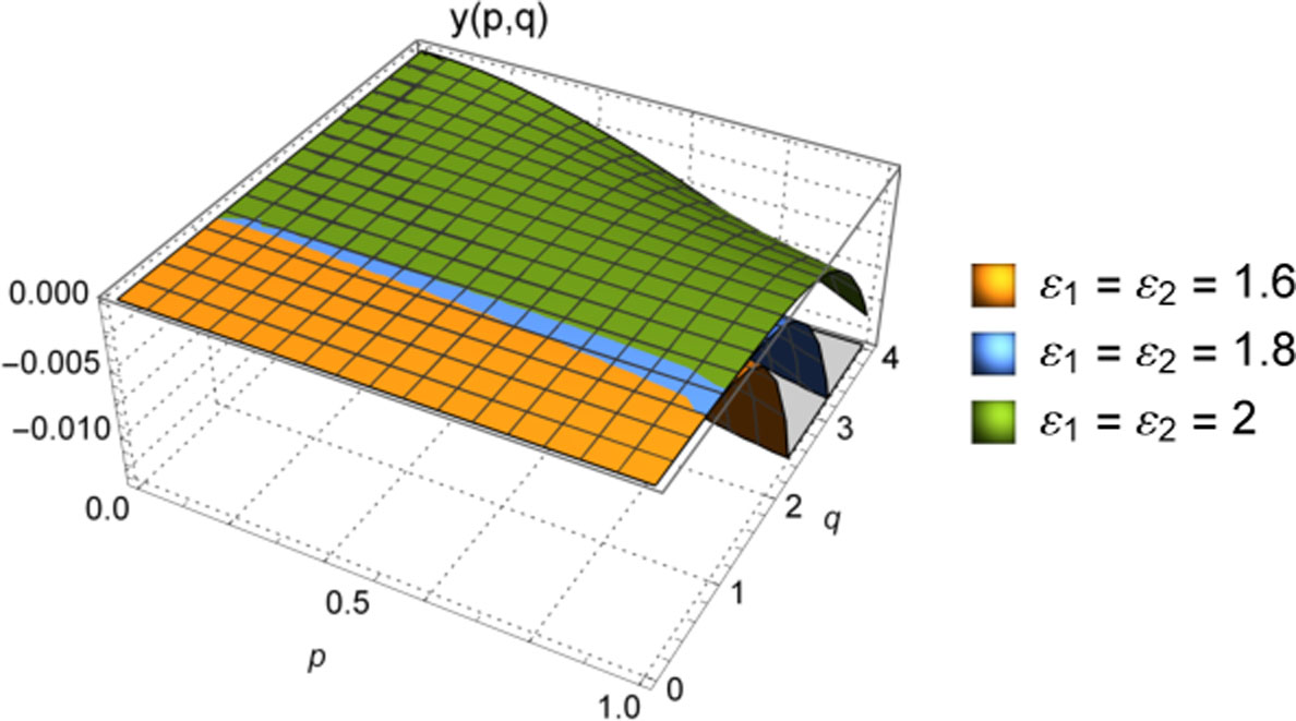
Fig. 1
The approximate graphs of Eq. (51) for the values u = v = 0,1,2,3, κ = μ = 1, σ = τ = 3, 0 < p < 1, 0 < q < 4, ɛ1 = ɛ2 = 1.6 (yellow), ɛ1 = ɛ2 = 1.8 (blue) and ɛ1 = ɛ2 = 2 (green).
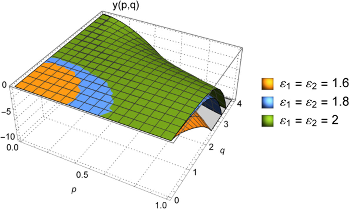
Fig. 2
The approximate graphs of Eq. (52) for the values u = v = k = 0,1,2,3, κ = μ = ϑ1 = 1, ϑ2 = 2, ϑ3 = 5, z = 0.5, 0 < p < 1, 0 < q < 4, ɛ1 = ɛ2 = 1.6 (yellow), ɛ1 = ɛ2 = 1.8 (blue) and ɛ1 = ɛ2 = 2 (green).
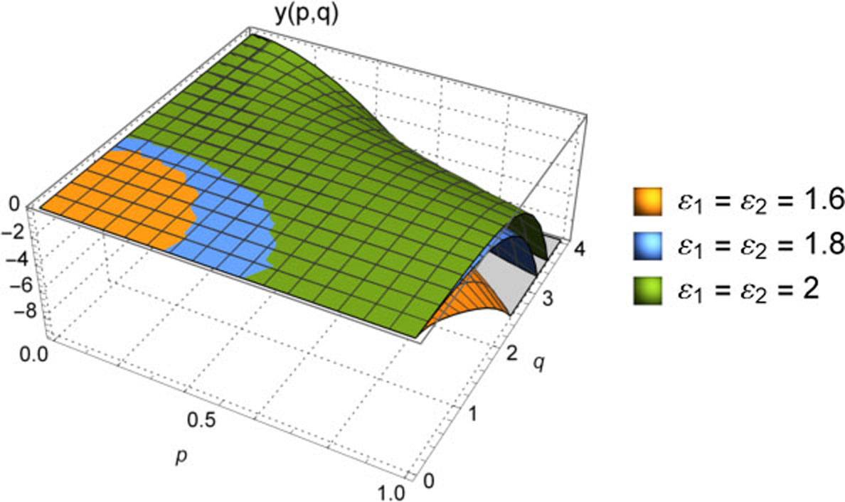
Fig. 3
The approximate graphs of Eq. (53) for the values u = v = k = 0,1,2,3, κ = μ = 1, ϑ2 = 2, ϑ3 = 5, z = 0.5, 0 < p < 1, 0 < q < 4, ɛ1 = ɛ2 = 1.6 (yellow), ɛ1 = ɛ2 = 1.8 (blue) and ɛ1 = ɛ2 = 2 (green).
Application 5.5
We let the general kernel as follows
So the fractional partial differential equation for Application (5.2) is
the fractional partial differential equation for Application (5.3) is the fractional partial differential equation for Application (5.4) isThen the solution of the first fractional partial differential equation is
the solution of the second fractional partial differential equation is the solution of the third fractional partial differential equation is6. Beta distribution with general kernel
One of the application areas of various generalized beta functions is statistics. The beta distribution is a continuous probability distribution that is widely used in Bayesian statistics and in modelling ratios and proportions. The beta function with general kernel is a general function that encompasses various beta functions that find applications in various fields such as physics, engineering and finance. Now we give the beta distribution with general kernel and describe the incomplete beta function with general kernel.
Application 6.1
We give the beta distribution with general kernel by
If λ ∈ ℝ, then for −∞ < σ< ∞, −∞ < τ< ∞
The variance of the distribution is
The moment generation function of the distribution is
The cummulative distribution of F(ω) can be written as
where is incomplete beta function with general kernel.7. Conclusions and remarks
In this paper, we introduced the gamma, beta, Gauss hypergeometric and confluent hypergeometric functions with general kernel. We also examined that special functions with general kernel generate other special functions in literature. Furthermore, we gave fundamental properties and presented some applications of special functions with general kernel. Finally, we obtained the incomplete beta function with general kernel by defining the beta distribution with general kernel. We conclude this paper by stating that in future works we will introduce their new structures with general kernel of various special functions such as Horn, Appell, Lauricella, Srivastava and also their new structures with general kernel of various fractional operators such as Riemann-Liouville, Caputo, Kober-Erdelyi and give their various potential properties and applications.
8. Declarations
8.1. Conflict of interest
The authors hereby declare that there is no conflict of interests regarding the publication of this paper.
8.2. Funding
Not applicable.
8.3. Author’s Contribution
E.A.-Writing-Original Draft. İ.O.K.-Writing, Review and Editing.
8.4. Acknowledgement
This study was partly presented in the V. International Turkic World Congress on Science and Engineering (TURK-COSE-2023) which organized by Kyrgyz-Turkish Manas University on September 15-17, 2023 in Bishkek-Kyrgyzstan. Many thanks to Editor-in-Chief Prof. Dr. Haci Mehmet Baskonus for his guidelines and opinions throughout this process.
8.5. Data availability statement
All data that support the findings of this study are included within the paper.
8.6. Using of AI tools
The authors declare that they have not used Artificial Intelligence (AI) tools in the creation of this article.