
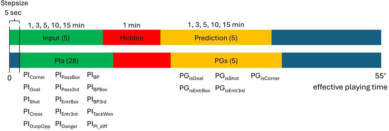
Figure 1.
Visualization of the In-Play Prediction Masking approach, the rolling window approach, and the utilized PIs; PGs; IW and PW window sizes. The lower band visualizes the rolling window, whereas all windows moved one step further. In brackets the number of configuration feature levels.
Table 1:
a) Performance indicators (PIs) and b) Prediction goals (PGs) of a team and their definitions utilized in our study. PIs 1–14 as individual PIs and 15–28 as the difference to the opponent team of the individual ones. The definition of a PI is always based on the performance of the respective team in an interval and is either an event performed, or a metric based on actions of the team. The definition of a PG is that the event happens at minimum once in the respective prediction window for the team.
| No | Abbreviation | Definition |
|---|---|---|
| a) Performance Indicators (PI) | ||
| 1 | PICorner | Number of corner kicks |
| 2 | PIEntrBox | Number of entries of a player with ball possession into the opponent box |
| 3 | PIEntr3rd | Number of entries of a player with ball possession into the attacking third |
| 4 | PIGoal | Number of goals scored |
| 5 | PIShot | Number of shot attempts |
| 6 | PICross | Number of crosses |
| 7 | PITackWon | Number of tacklings won |
| 8 | PIPassBox | Number of successful passes in or into the opponent box |
| 9 | PIPass3rd | Number of successful passes in or into the attacking third |
| 10 | PIBP | Time of ball possession |
| 11 | PIBPBox | Time of ball possession in the box |
| 12 | PIBP3rd | Time of ball possession in the attacking third |
| 13 | PIOutpOpp | Number of outplayed opponent players by successful passes |
| 14 | PIDanger | Goal scoring probability at each moment (Link et al., 2016) |
| 15-28 | PIPI_diff | Difference of both PI values, (Team – Opponent) |
| b) Prediction Goals (PG) | ||
| 1 | PGisGoal | A goal event for the team occurs |
| 2 | PGisShot | A shot event for the team occurs |
| 3 | PGisCorner | A corner kick event for the team occurs |
| 4 | PGisEntrBox | An entry into the opponent box performed by the team occurs |
| 5 | PGisEntr3rd | An entry into the attacking third performed by the team occurs |
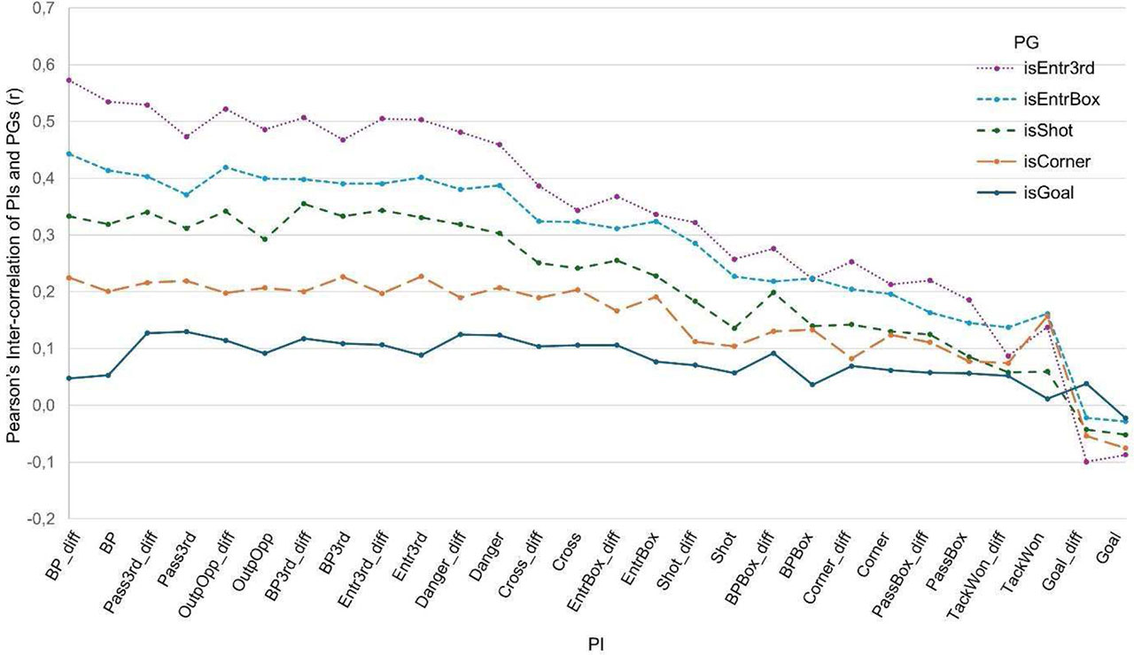
Figure 2.
Pearson’s inter-correlation of PIs and PGs with a window size of 15 minutes ordered for readability. Complete results are shown in Table 3 in the Appendix.
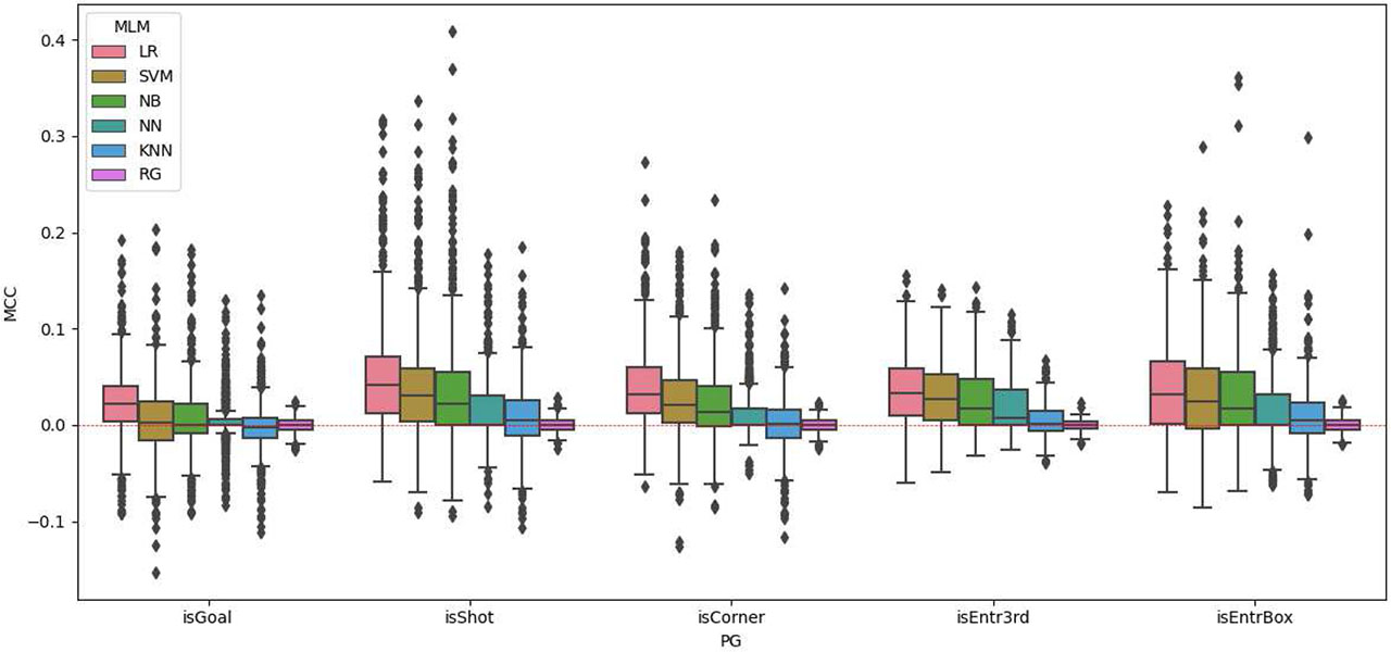
Figure 3.
MCC results of all experiments split by MLMs and PGs. Each boxplot contains results of 700 experiments, except for the PGisEntr3rd with 250 experiments. The red dotted line indicates MCC=0.
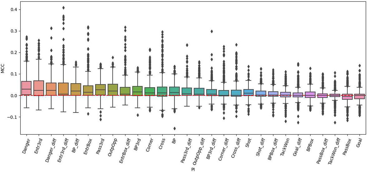
Figure 4.
MCC results of all experiments split by PIs. Each boxplot contains the results of 545 experiments. Boxplots are sorted by their MCCmean in descending order. The red dotted line indicates MCC=0.
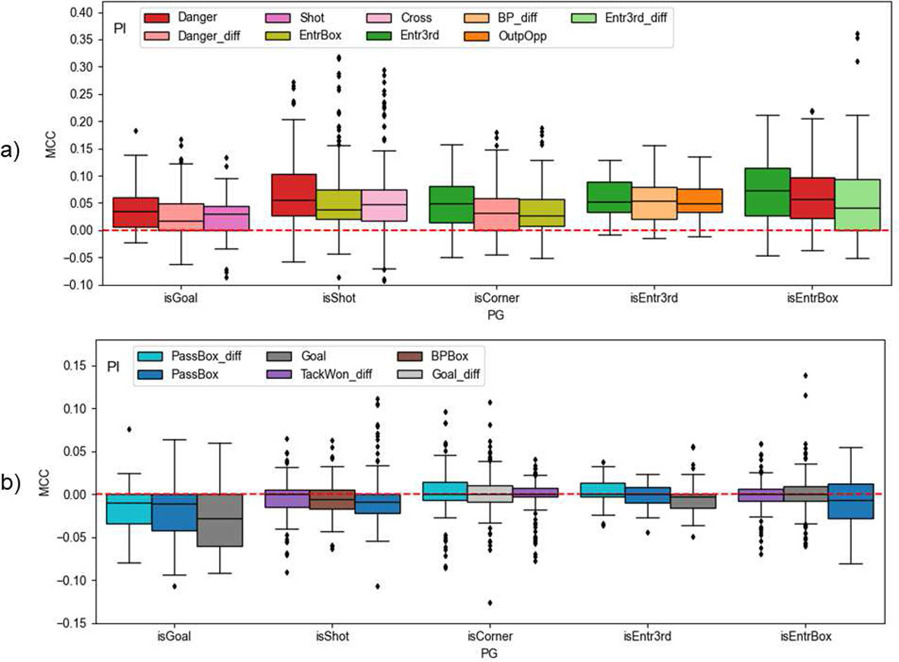
Figure 5.
a) Top 3 and b) Bottom 3 PIs for each PG. PIs are sorted by their mean MCC results in descending order. Each boxplot contains the results of 125 experiments, except for the PGisEntr3rd with 45 experiments. The red dotted line indicates MCC=0.
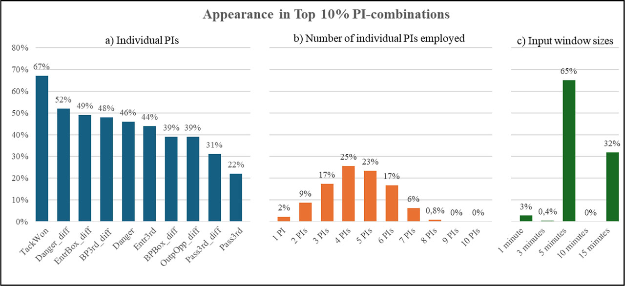
Figure 6.
The percentual appearance in the Top 10% PI-combinations in the application scenario (Part III) of a) the selected Top 10 individual Pls, b) the number of individual Pls combined, and c) the input window length.
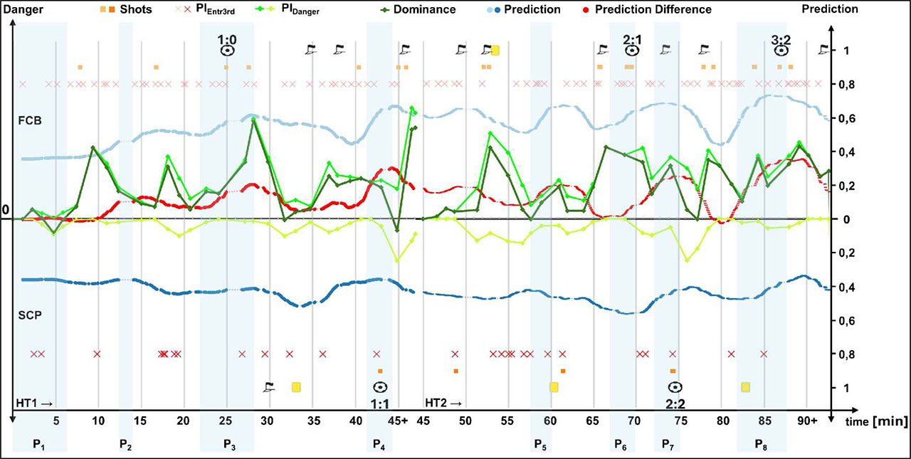
Figure 7.
Application of the trained model (rank 3) for an unseen match between FC Bayern Munich (FCB) vs SC Paderborn (SCP) in Season 19/20 which resulted in a 3:2. In the upper half (FCB) and the lower half (SCP) for each team important events (corner kicks, given cards, goals scored, shots taken), PIDanger and PIEntr3rd, and prediction values are illustrated over the course of the match. Also, Dominance by Link et al. (2016) and the goal prediction difference between both teams, as our proposed match momentum metric, are shown. Additionally, eight important sequences (P1-8) are highlighted.
Table 2:
An overview of the five utilized machine learning models applied with default configurations in the study and the minor individual changes in configuration that were determined as optimal in hyperparameter tuning experiments on subsets of the data.
| Machine Learning Model | Python library | Configuration | URL to documentation |
|---|---|---|---|
| Logistic Regression (LR) | Scikit-learn 1.4.0 |
| https://scikit-learn.org/stable/modules/generated/sklearn.linear_model.LogisticRegression.html#sklearn.linear_model.LogisticRegression |
| Gaussian Naive Bayes (NB) | Scikit-learn 1.4.0 | https://scikit-learn.org/stable/modules/generated/sklearn.naive_bayes.GaussianNB.html | |
| Support Vector Machine (SVM) | Scikit-learn 1.4.0 |
| https://scikit-learn.org/stable/modules/generated/sklearn.svm.SVC.html#sklearn.svm.SVC |
| K-Nearest-Neighbors (KNN) | Scikit-learn 1.4.0 |
| https://scikit-learn.org/stable/modules/generated/sklearn.neighbors.KNeighborsClassifier.html#sklearn.neighbors.KNeighborsClassifier |
| Neural Network (NN) | PyTorch 2.3.0 |
| https://pytorch.org/docs/stable/nn.html |
Table 3:
Pearson’s inter-correlation results of PIs and PGs for the window length of 15 minutes. Top 3 (green) and Bottom 3 (red) PIs per PG are highlighted. The best and worst results per PG are bold.
| PGisGoal | PGisCorner | PGisShot | PGisEntrBox | PGisEntr3rd | |
|---|---|---|---|---|---|
| PIBP_diff | .048 | .225 | .333 | .443 | .573 |
| PIBP | .053 | .201 | .319 | .414 | .535 |
| PIPass3rd_diff | .127 | .216 | .340 | .403 | .529 |
| PIPass3rd | .130 | .219 | .312 | .371 | .473 |
| PIOutpOpp_diff | .114 | .198 | .342 | .419 | .522 |
| PIOutpOpp | .092 | .207 | .292 | .400 | .486 |
| PIBP3rd_diff | .118 | .201 | .355 | .398 | .507 |
| PIBP3rd | .109 | .227 | .333 | .391 | .468 |
| PIEntr3rd_diff | .107 | .197 | .343 | .391 | .505 |
| PIEntr3rd | .089 | .227 | .331 | .401 | .503 |
| PIDanger_diff | .125 | .190 | .319 | .380 | .481 |
| PIDanger | .124 | .207 | .303 | .387 | .459 |
| PICross_diff | .104 | .190 | .251 | .324 | .387 |
| PICross | .106 | .204 | .242 | .323 | .343 |
| PIEntrBox_diff | .106 | .166 | .255 | .312 | .368 |
| PIEntrBox | .077 | .191 | .228 | .324 | .336 |
| PIShot_diff | .071 | .112 | .183 | .286 | .322 |
| PIShot | .057 | .104 | .136 | .227 | .258 |
| PIBPBox_diff | .092 | .130 | .199 | .218 | .276 |
| PIBPBox | .036 | .133 | .140 | .224 | .222 |
| PICorner_diff | .069 | .083 | .142 | .205 | .253 |
| PICorner | .062 | .124 | .130 | .196 | .213 |
| PIPassBox_diff | .058 | .111 | .125 | .164 | .220 |
| PIPassBox | .057 | .078 | .086 | .145 | .186 |
| PITackWon_diff | .052 | .074 | .058 | .138 | .087 |
| PITackWon | .012 | .157 | .060 | .162 | .138 |
| PIGoal_diff | .038 | −.054 | −.043 | −.022 | −.099 |
| PIGoal | −.022 | −.075 | −.052 | −.028 | −.087 |
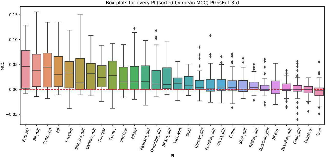
Figure 8.
Ranking of PIs for PGisEntr3rd. PIs are sorted by their mean MCC results in descending order. The red dotted line indicates MCC=0.
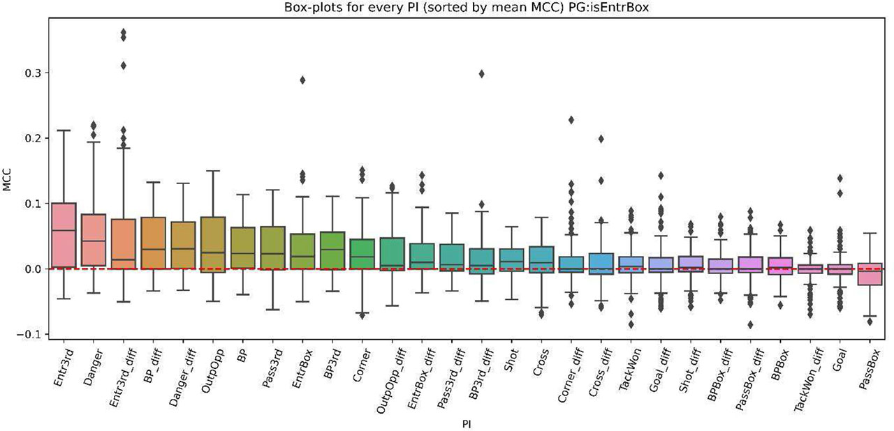
Figure 9.
Ranking of PIs for PGisEntrBox. PIs are sorted by their mean MCC results in descending order. The red dotted line indicates MCC=0.
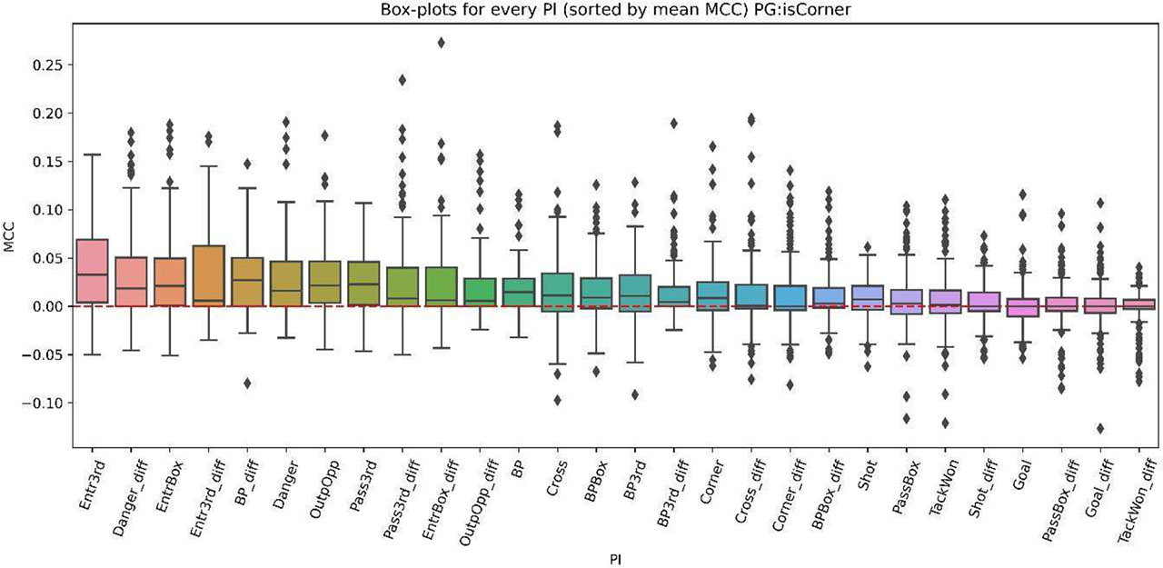
Figure 10.
Ranking of PIs for PGisCorner. PIs are sorted by their mean MCC results in descending order. The red dotted line indicates MCC=0.
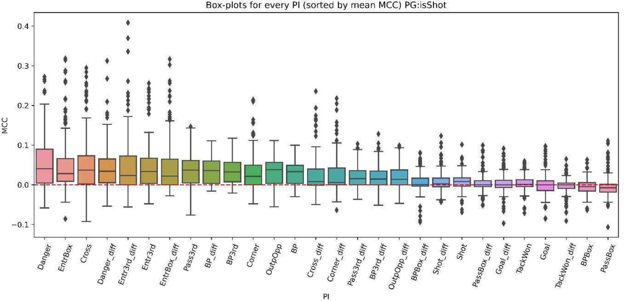
Figure 11.
Ranking of PIs for PGisShot. PIs are sorted by their mean MCC results in descending order. The red dotted line indicates MCC=0.
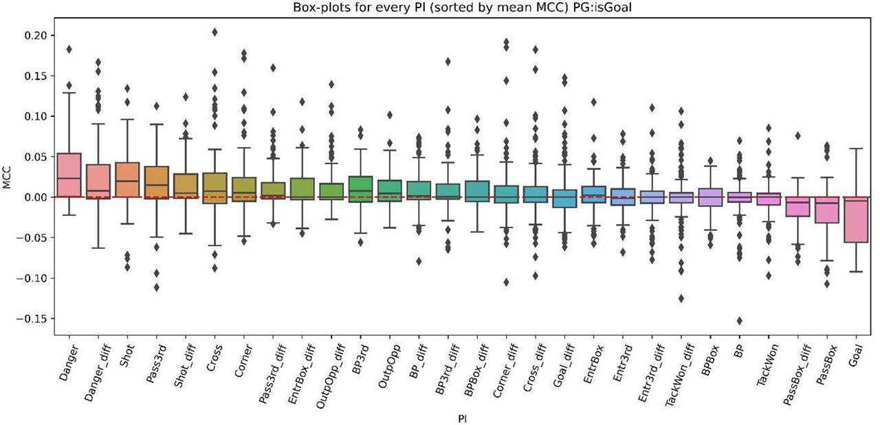
Figure 12.
Ranking of PIs for PGisGoal. PIs are sorted by their mean MCC results in descending order. The red dotted line indicates MCC=0.
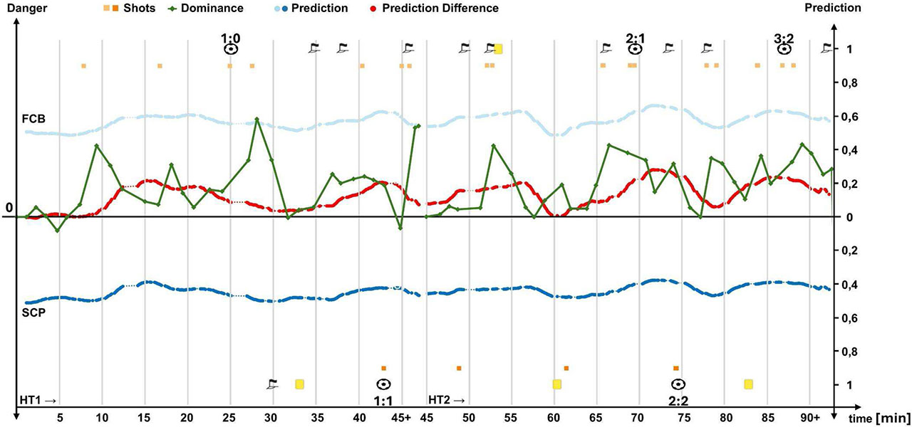
Figure 13.
Application of the 1st ranked model for an unseen match between FC Bayern Munich (FCB) vs SC Paderborn (SCP) in Season 19/20 which resulted in a 3:2. In the upper half (FCB) and the lower half (SCP) for each team important events (corner kicks, given cards, goals scored, shots taken), Dominance by Link et al. (2016) and the prediction difference, as our proposed match momentum metric, are shown.
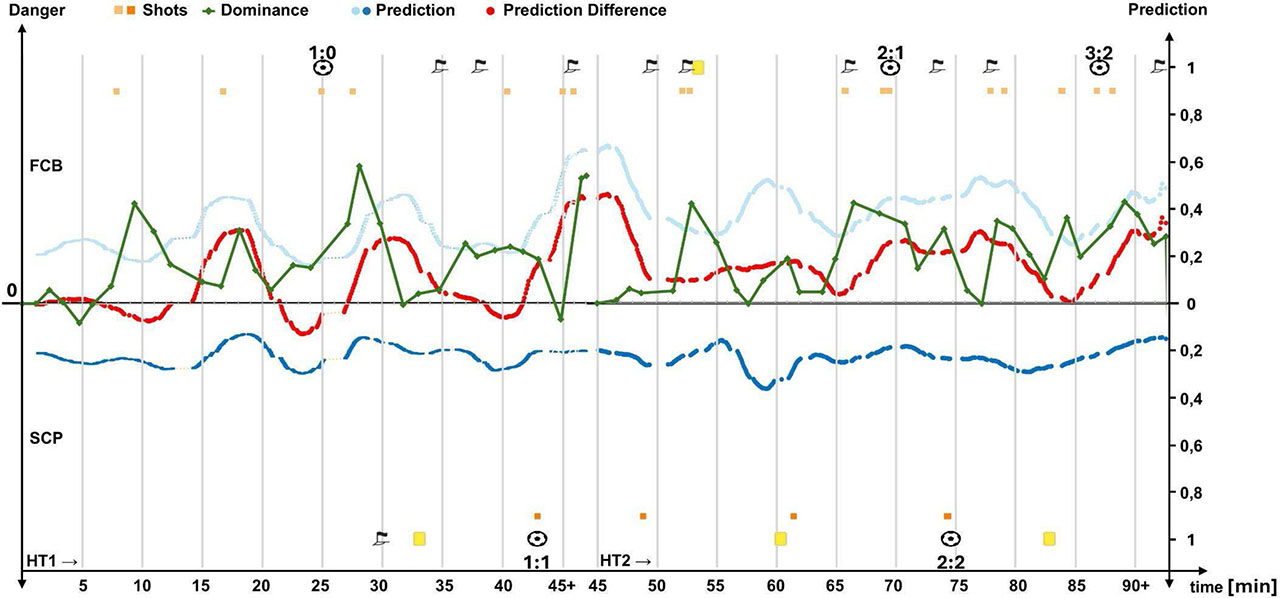
Figure 14.
Application of the 2nd ranked model for an unseen match between FC Bayern Munich (FCB) vs SC Paderborn (SCP) in Season 19/20 which resulted in a 3:2. In the upper half (FCB) and the lower half (SCP) for each team important events (corner kicks, given cards, goals scored, shots taken), Dominance by Link et al. (2016) and the prediction difference, as our proposed match momentum metric, are shown.