
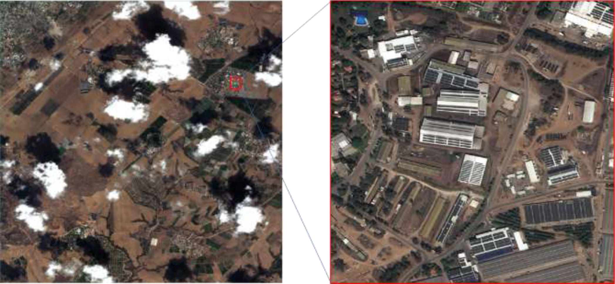
Figure 1.
Shows remote sensing portraits. The left portrait is the original image, which contains a lot of information. The right image is a partial image captured from the left image. It can be seen that even if it is magnified many times, the information in the image is still very rich
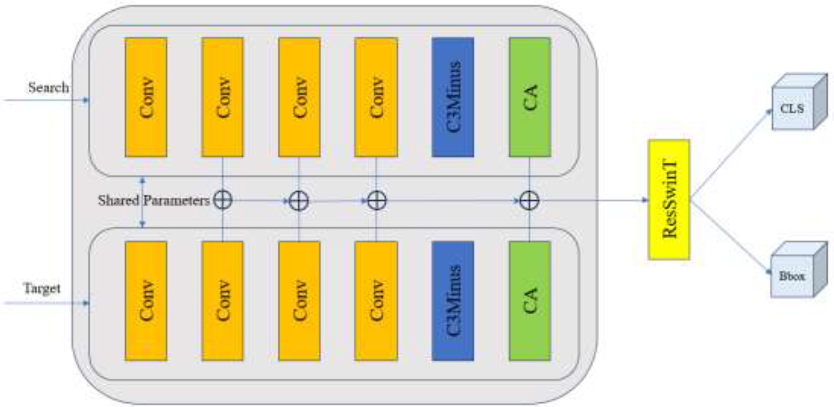
Figure 2.
Network Structure. The proposed network's architecture is organized into three main components: the Backbone, the ResSwinT module, and the regression head. The Backbone is constructed upon the ResNet-50 architecture, with significant enhancements that include the incorporation of C3Minus and CA modules. These additions are designed to enhance the ability to extract features. The network effectively fuses the outputs from three distinct convolutional layers along with the outputs from the CA module. This fused information is subsequently passed to the ResSwinT module, which processes the data to generate hierarchical feature representations. Finally, the output from the ResSwinT module is directed to the regression head, which is responsible for accurately locating the target object in the image.
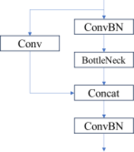
Figure 3.
C3Minus network structure. The network consists of three convolution layers and one BottleNeck layer. ConvBN refers to the Batch Normalization and activation function, and Concat is a short circuit
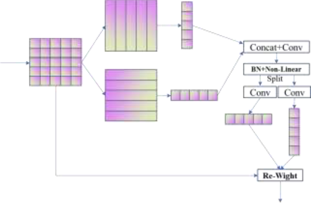
Figure 4.
CA network structure. The entire module performs average pooling in the horizontal and vertical directions, then uses Transform to encode the spatial information, and finally fuses the spatial information by weighting it on the channel, making the network's overall perception of space more profound.
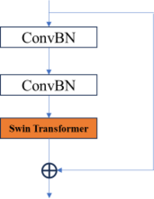
Figure 5.
ResSwinT network structure, the overall structure uses a RestNet module as the basis, adds a Swin Transformer layer, and further extracts and fuses image features.
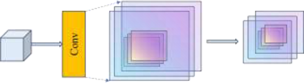
Figure 6.
Depth-wise Cross Correlation
TABLE I.
Experimental Environment
| Experimental Environment | Version |
|---|---|
| CPU | Intel Xeon E5-2698 |
| GPU | NVIDIA Tesla V100 32G |
| Language | Python 3.8 |
| Framework | Pytorch |
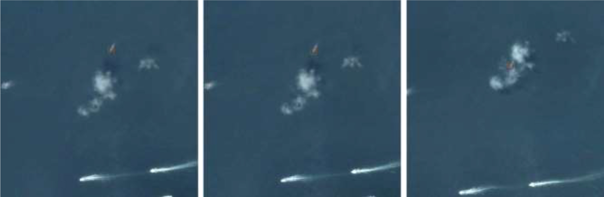
Figure 7.
Experimental results. The red part is the model result and the green part is the real frame.
TABLE II.
The success rate and accuracy of this method are compared with the SOTA method. The red value in the table is highest, and green value is second highest.
| Models | Years | precision | success |
|---|---|---|---|
| SiamRPN | 2018 | 0.753 | 0.342 |
| SiamRPN++ | 2018 | 0.435 | 0.261 |
| SiamMask | 2019 | 0.569 | 0.278 |
| SiamBAN | 2020 | 0.784 | 0.497 |
| SiamCar | 2022 | 0.769 | 0.502 |
| Ours | - | 0.803 | 0.549 |