
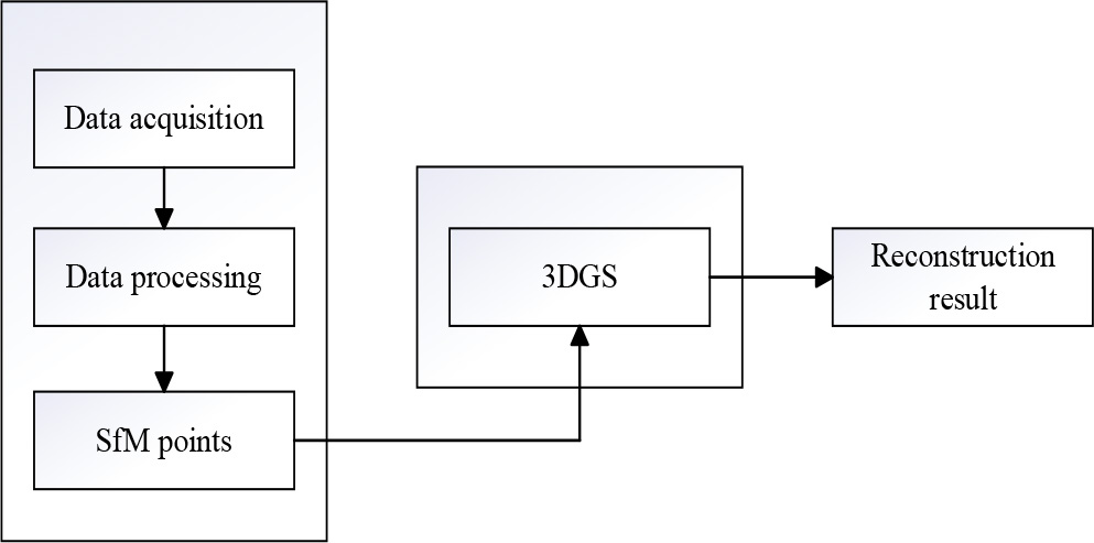
Figure 1.
3D Reconstruction Process Map.
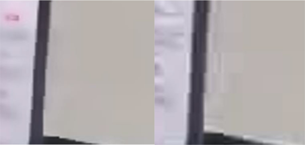
Figure 2.
The result of adding bilateral filters for indoor scenes.
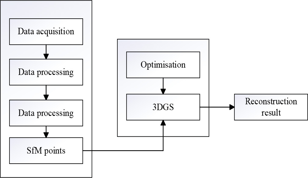
Figure 3.
Optimized 3D Reconstruction Process Map.
TABLE I.
Experimental Results
| Dataset | PSNR | SSIM | ||
|---|---|---|---|---|
| 3DGS | ours | 3DGS | ours | |
| office0 | 38.45 | 39.05 | 0.925 | 0.934 |
| office1 | 36.97 | 37.17 | 0.938 | 0.954 |
| office2 | 36.39 | 36.68 | 0.945 | 0.962 |
| office3 | 35.85 | 36.35 | 0.941 | 0.958 |
| office4 | 36.54 | 36.66 | 0.939 | 0.941 |
| room0 | 37.26 | 38.06 | 0.915 | 0.923 |
| rooml | 36.28 | 37.75 | 0.929 | 0.935 |
| room2 | 34.98 | 35.14 | 0.913 | 0.927 |
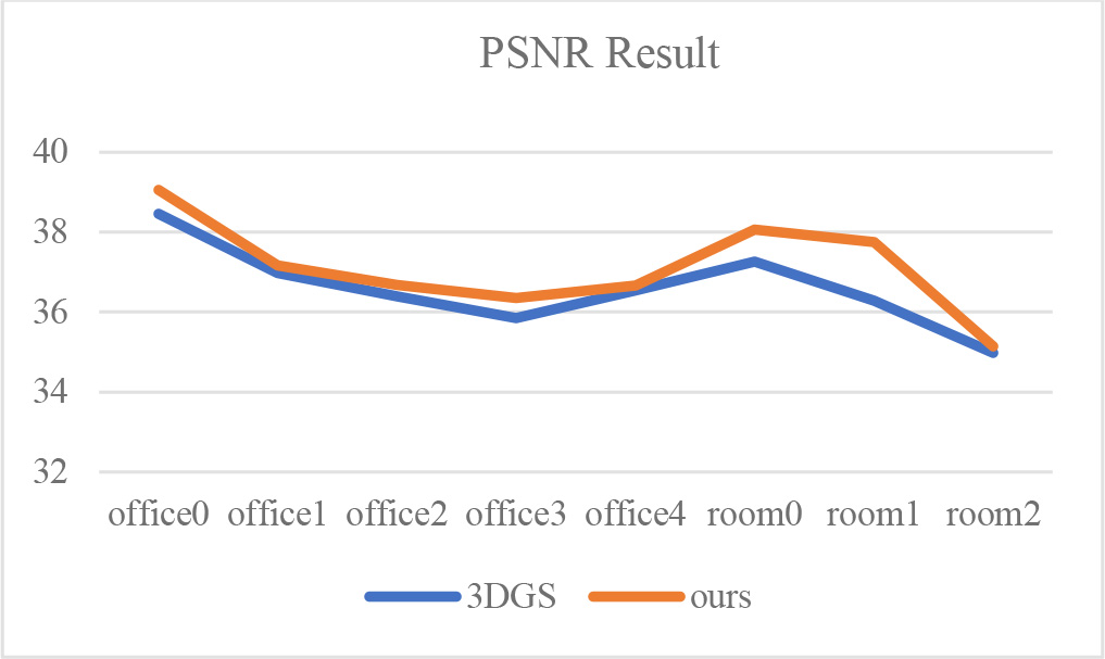
Figure 4.
Performance of peak signal-to-noise ratios of 3DGS and ours models for eight different indoor scenes, respectively.
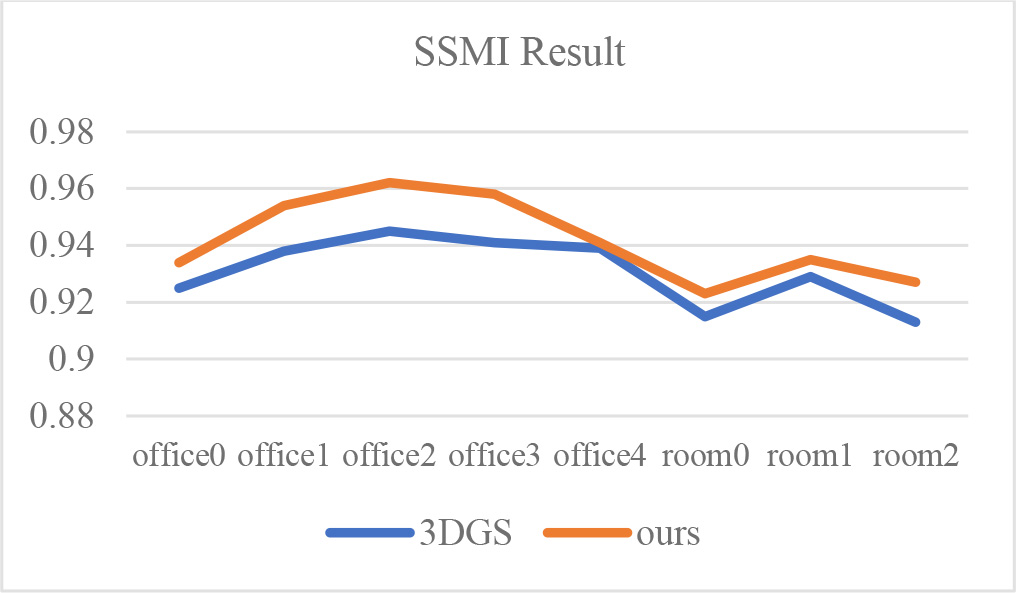
Figure 5.
Representation of structural similarity between 3DGS and ours model for 8 different indoor scenes, respectively.