
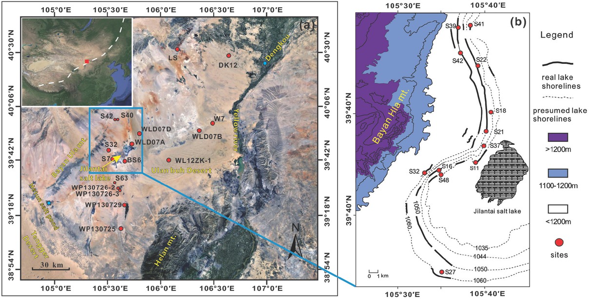
Fig 1
Regional setting (a) and sampling sites (b) (modified from Chen et al., 2008). The inset in the left upper corner of (a) is a remote sensing image of East Asia showing the location of the study area (marked by square) and the modern monsoon limit.
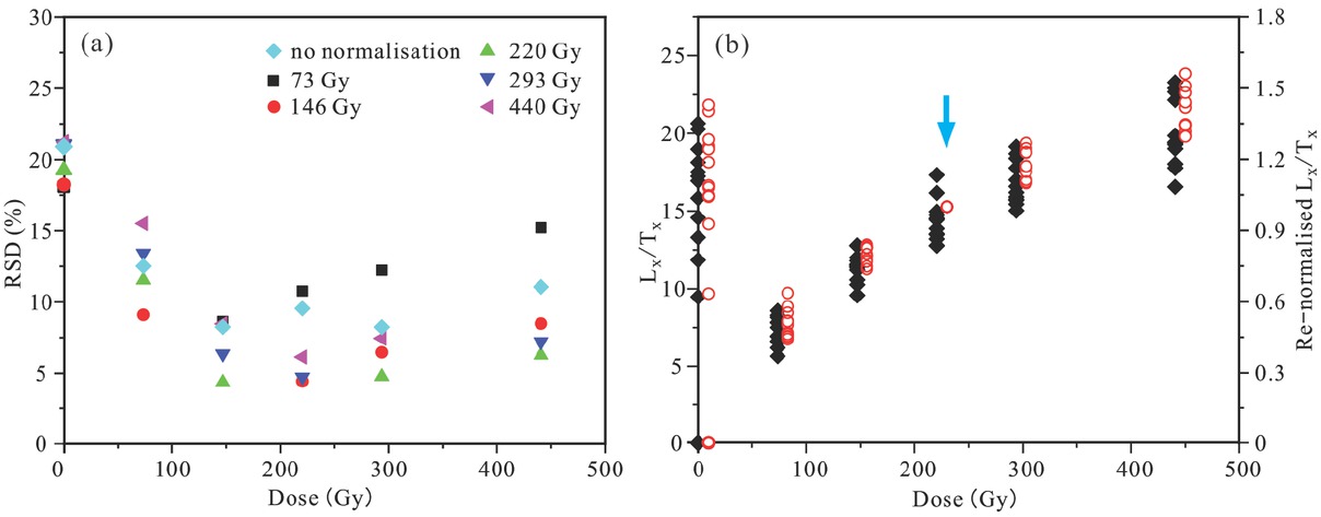
Fig 2
(a) Relative standard deviation (RSD) of the sensitivity-corrected natural signal (Ln/Tn) and re-normalised regenerative-dose signals (Lx/Tx) of representative sample LS-4 (the diamond symbol), plotted versus the regenerative doses. (b) Plots of the sensitivity-corrected natural signal (Ln/Tn) and regenerative dose signal (Lx/Tx) (filled black diamonds) (left-hand axis) versus the regenerative dose, and plots of the re-normalised signals with the extra regenerative dose of 220 Gy (red circles) which are plotted using an offset of a few Gy offset to the right on the x-axis for clarity (right-hand axis).
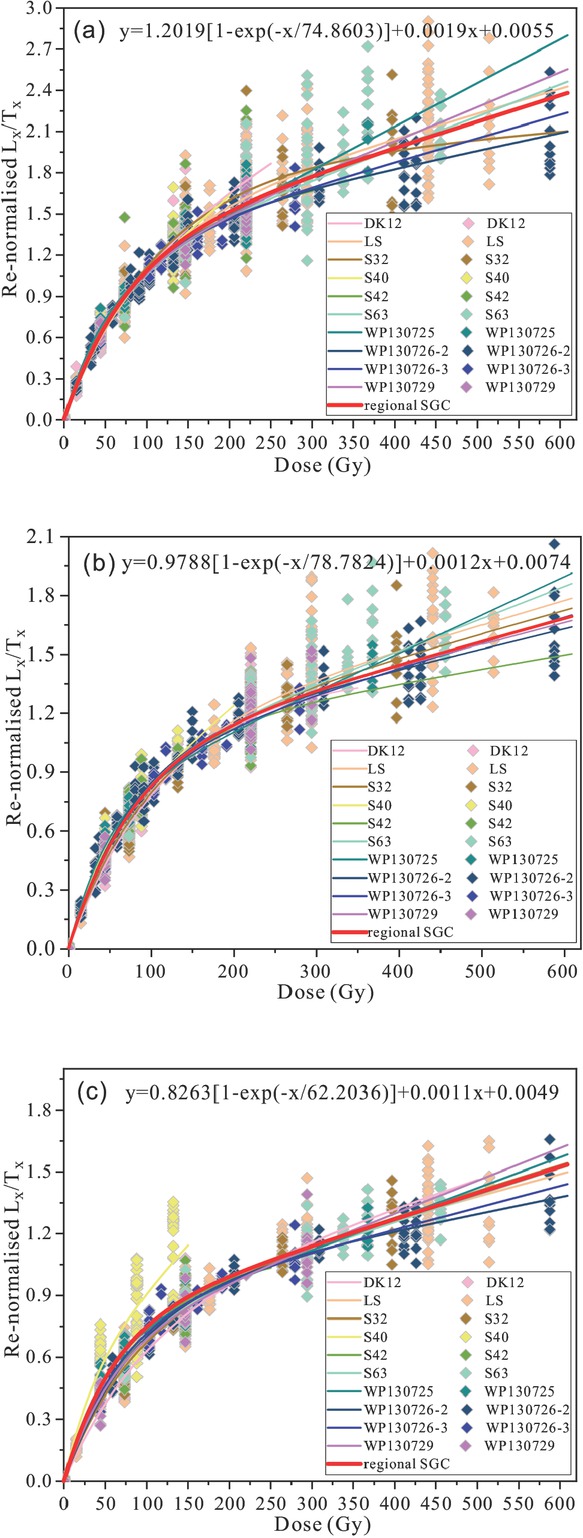
Fig 3
Comparison of the re-normalisation results with OSL signals of the re-normalisation dose of (a) 88 Gy, (b) 147 Gy and (c) 220 Gy.
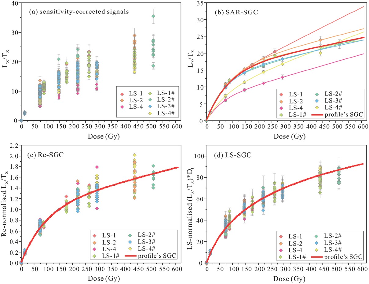
Fig 4
Comparison of re-normalised OSL signals (b, c and d) with the sensitivity-corrected OSL signals (a) from samples from the LS profile. Illustration of the potential SGCs established using (b) SAR-SGC, (c) Re-SGC and (d) LS-SGC methods. The diamonds represent the OSL signals of different samples, and the red curve represents the fitted SGC. In (b), the potential SGCs of different profiles are shown using the same colour as in the legend in Fig. 4-4b.
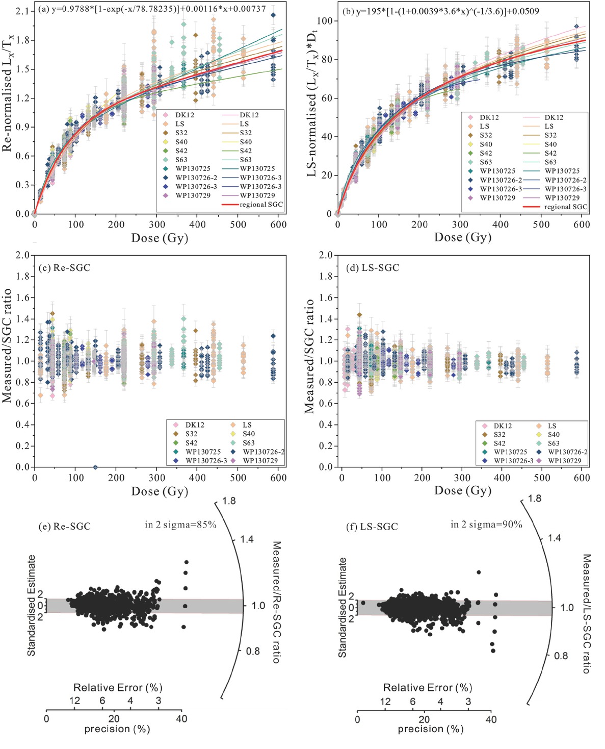
Fig 5
(a) The regional SGC (red curve) and DRCs from samples of profiles (the other coloured curves) established using the Re-SGC method. (b) The regional SGC (red curve) and DRCs of profiles (the other coloured curves) established using the LS-SGC method. (c) Ratios between the re-normalised data and the Re-SGC in (a), plotted against regenerative dose. (d) Ratios between the LS-normalised data and the LS-SGC in (b), plotted against regenerative dose. (e) Radial plot of the ratios shown in (c). (f) Radial plot of the ratios shown in (d). In the plots (e) and (f), the relatively high precision of 5–6 points, which scatter from the rest of the data points, was caused by OSL signal saturation.
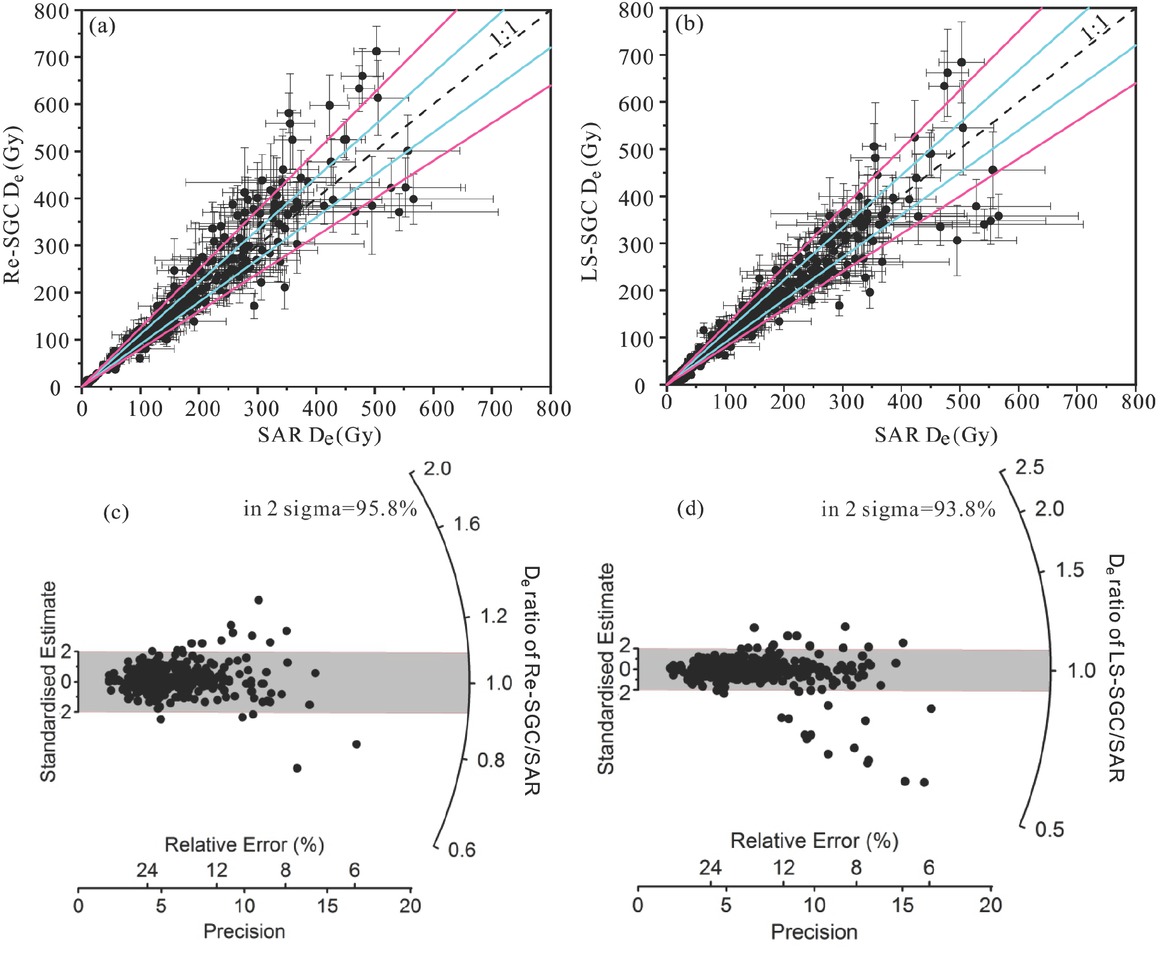
Fig 6
Comparison of De values obtained using the SAR protocol with those obtained using the Re-SGC (a) and LS-SGC (b) methods. The dashed black line is the 1:1 line, the solid blue lines define the 10% error range, and the solid pink lines define the 20% error range. (c) Radial plot showing ratios of the Re-SGC De values to the SAR De. (d) Radial plot showing the ratios of the LS-SGC De values to the SAR De. In the plot (d), 10 points with very low ratio were caused by OSL signal saturation.
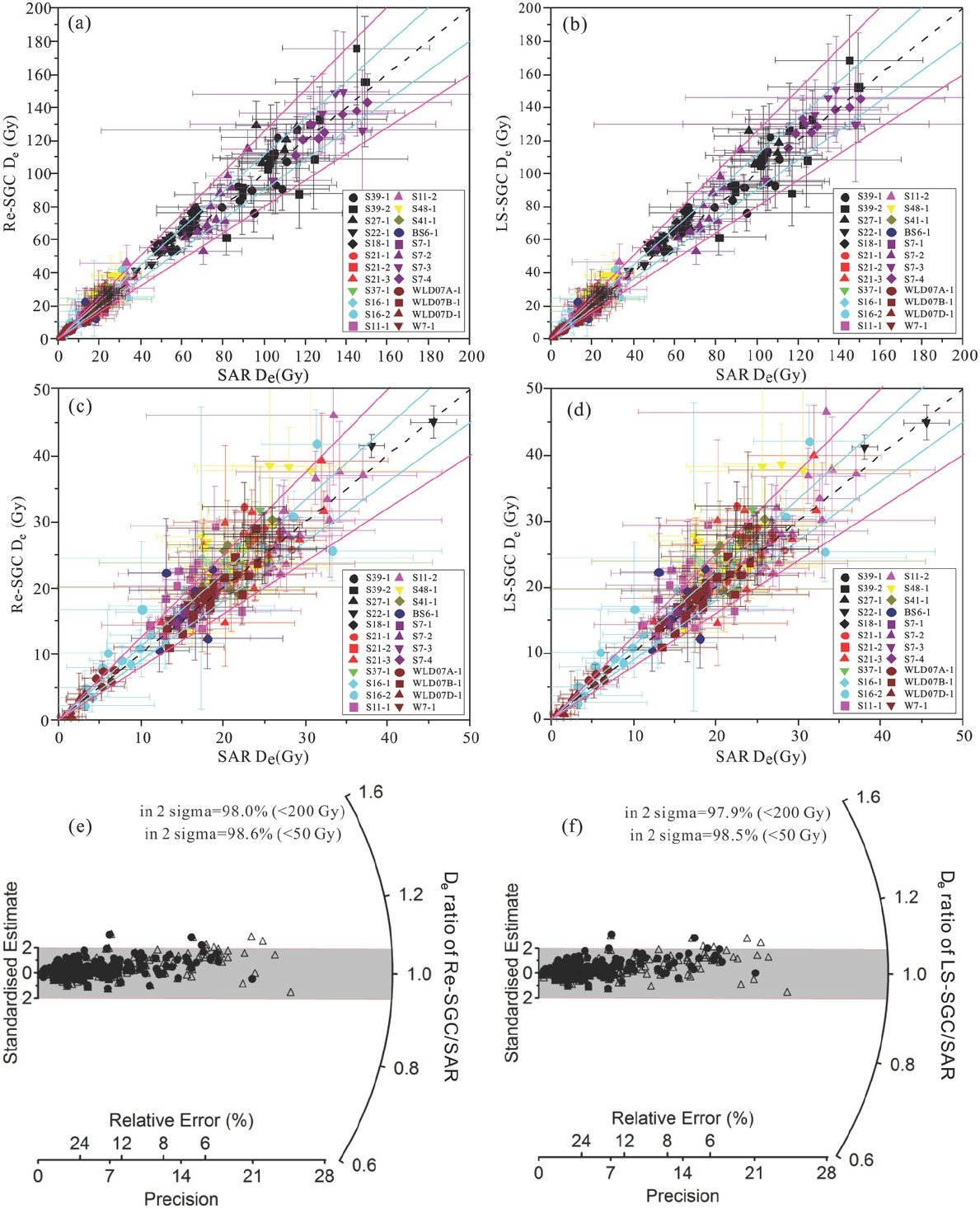
Fig 7
Comparison of De values obtained using the SAR protocol with those obtained using the regional SGCs established using the Re-SGC (a and c) and LS-SGC (b and d) methods, for samples which were not used in the establishment of the regional SGCs. In these plots, the black dashed lines are the 1:1 ratio, and the areas enclosed by the blue solid lines are the 10% error range of unity, and the areas enclosed by the pink solid lines are the 20% error range of unity. (e) Radial plot showing the ratios of the Re-SGC De values to the SAR De. (f) Radial plot showing the ratios of the LS-SGC De values to the SAR De. Within (e) and (f), the data within 200 Gy are shown as open triangles and those <50 Gy as filled circles.
Table S1
The double SAR protocol applied in measuring OSL signals in this study.
| Step | Operation | Measured |
|---|---|---|
| 1 | Regeneration dose di (i=0,1,2,3,4,5) | d0=0, d1=d4 |
| 2 | Preheat @160–260°C for 10 s | |
| 3 | OSL @50°C for 40 s | Lx |
| 4 | OSL @125°C for 40 s | |
| 5 | Test dose 20–100 s | |
| 6 | TL 160–220°C | Tx |
| 7 | OSL @50°C for 40 s | |
| 8 | OSL @125°C for 40 s | |
| 9 | Illumination @280°C for 100 s |
Table S2
A summary of studied samples, including their locations, sedimentary types and grain size and measurement conditions in measuring OSL signals of quartz in this study.
| Profile/Core | Sample | Location | Sediment type | Grain size (μm) | Preheat/cut-heat (°C) | Test dose (s) | Number of aliquots | Data source |
|---|---|---|---|---|---|---|---|---|
| DK-1 | Lacustrine | 180-250 | 200/160 | 100 | 10 | |||
| DK-2 | Lacustrine | 180-250 | 160/160 | 100 | 11 | |||
| DK-3 | Lacustrine | 180-250 | 180/160 | 100 | 12 | |||
| DK-4 | N40°23′14.3″, | Lacustrine | 180-250 | 200/160 | 100 | 11 | ||
| DK12 | DK-5 | E106°40′12.0″ | Lacustrine | 180-250 | 220/160 | 100 | 12 | (Fan et al., 2017) |
| DK-6 | Lacustrine | 180-250 | 180/160 | 100 | 12 | |||
| DK-7 | Lacustrine | 180-250 | 260/160 | 100 | 11 | |||
| DK-1# | Lacustrine | 180-250 | 200/160 | 50 | 7 | |||
| DK-2# | Lacustrine | 180-250 | 160/160 | 100 | 6 | |||
| LS-1 | Lacustrine | 90-125 | 160/160 | 30 | 8 | |||
| LS-2 | Lacustrine | 90-125 | 180/160 | 30 | 5 | |||
| LS-3 | Lacustrine | 90-125 | 200/160 | 30 | 12 | |||
| LS-4 | N40°26′22.88″, | Lacustrine | 90-125 | 260/160 | 30 | 11 | ||
| LS | LS-1# | E106°11′36.26″ | Lacustrine | 90-125 | 160/160 | 30 | 12 | (Zhang 2016) |
| LS-2# | Lacustrine | 90-125 | 180/160 | 30 | 10 | |||
| LS-3# | Lacustrine | 90-125 | 200/160 | 30 | 10 | |||
| LS-4# | Lacustrine | 90-125 | 260/160 | 30 | 11 | |||
| S32 | S32-1 S32-2 | N39°44′01.0″, E105°33′22.0″ | Lacustrine Lacustrine | 90-125 90-125 | 160/160 260/160 | 30 30 | 8 10 | (Zhang 2016) |
| S40-1 | Lacustrine | 90-125 | 200/160 | 50 | 16 | |||
| S40 | S40-2 | N39°56′55.10″, E105°38′07.50 ″ | Lacustrine | 90-125 | 180/160 | 50 | 11 | (Zhang 2015) |
| S40-3 | Lacustrine | 90-125 | 260/160 | 50 | 10 | |||
| S42-1 | Lacustrine | 90-125 | 180/160 | 50 | 9 | |||
| S42 | S42-2 | N39°56′54.58″, | Lacustrine | 90-125 | 240/160 | 50 | 8 | (Zhang 2015) |
| E105°37′5.51″ | ||||||||
| S42-3 | Lacustrine | 90-125 | 180/160 | 50 | 12 | |||
| S63-1 | Lacustrine | 90-125 | 200/160 | 50 | 10 | |||
| S63 | S63-2 S63-3 | N39°30′15.7″, E105°36′32.2″ | Lacustrine Lacustrine | 90-125 90-125 | 220/160 160/160 | 50 50 | 4 8 | This work |
| S63-2# | Lacustrine | 90-125 | 220/160 | 50 | 11 | |||
| WP130725 | WP130725-1 WP130725-2 | N39°10′56.64″, E105°39′38.92″ | Fluvial Fluvial | 90-125 90-125 | 160/160 160/160 | 50 50 | 14 6 | (Zhang 2015) |
| WP130726-2-1 | Fluvial | 90-125 | 180/160 | 50 | 11 | |||
| WP130726-2 | WP130726-2-2 | N39°27′57.68″, E105°38′17.24 ″ | Fluvial | 90-125 | 160/160 | 50 | 11 | This work |
| WP130726-2-3 | Fluvial | 90-125 | 220/160 | 50 | 11 | |||
| WP130726-3 | WP130726-3-1 WP130726-3-2 | N39°27′3.79″, E105°39′5.79″ | Fluvial Fluvial | 90-125 90-125 | 240/160 220/160 | 50 50 | 9 12 | This work |
| WP130729-1 | N39°20′50.5″, | Fluvial | 90-125 | 240/160 | 50 | 16 | ||
| WP130729 | WP130729-2 | E105°41′52.7″ | Fluvial | 90-125 | 180/160 | 50 | 12 | (Zhang 2015) |
| S39 | S39-1 | N39°58′32″, | Lacustrine | 106-180 | 260/220 | 80 | 15 | (Fan 2008) |
| S39-2 | E105°37′07″ | Lacustrine | 150-180 | 260/220 | 80 | 12 | ||
| N39°34′14″, | ||||||||
| S27 | S27-1 | E105°35′37″ | Lacustrine | 90-125 | 260/160 | 100 | 6 | (Fan 2008) |
| N39°52′14″, | ||||||||
| S22 | S22-1 | E105°39′45″ | Lacustrine | 90-125 | 260/160 | 50 | 13 | (Fan 2008) |
| N39°47′53″, | ||||||||
| S18 | S18-1 | E105°39′58″ | Lacustrine | 90-125 | 260/220 | 50 | 22 | (Fan 2008) |
| S21-1 | Lacustrine | 180-300 | 260/160 | 50 | 15 | |||
| S21 | S21-2 | N39°47′01″, E105°39′24 ″ | Lacustrine | 90-125 | 260/160 | 20 | 16 | (Fan 2008) |
| S21-3 | Lacustrine | 300-500 | 260/160 | 80 | 11 | |||
| N39°46′45″, | ||||||||
| S37 | S37-1 | E105°39′34″ | Lacustrine | 125-180 | 260/160 | 20 | 12 | (Fan 2008) |
| S16-1 | N39°44′11″, | Lacustrine | 90-125 | 260/160 | 50 | 6 | ||
| S16 | S16-2 | E105°34′24″ | Lacustrine | 250-300 | 260/220 | 50 | 29 | (Fan 2008) |
| S11 | S11-1 | N39°44′57″, | Lacustrine | 180-300 | 260/160 | 20 | 16 | (Fan 2008) |
| S11-2 | E105°38′40″ | Lacustrine | 90-125 | 260/220 | 20 | 28 | ||
| S48 | S48-1 | N39°44′03″, | Lacustrine | 250-300 | 260/160 | 20 | 18 | (Fan 2008) |
| E105°34′24″ | ||||||||
| S41 | S41-1 | N39°58′12″, E105°38′29 ″ | Lacustrine | 500-1000 | 260/220 | 50 | 7 | (Fan 2008) |
| N39°39′39″, | ||||||||
| BS6 | BS6-1 | E105°40′54″ | Dune | 90-125 | 260/160 | 20 | 9 | (Fan et al., 2010) |
| S7-1 | Dune | 90-125 | 260/160 | 20 | 9 | |||
| S7-2 | N39°39′53″, | Dune | 125-150 | 260/220 | 80 | 13 | ||
| S7 | S7-3 | E105°36′17″ | Dune | 125-150 | 260/220 | 50 | 6 | (Fan et al., 2010) |
| S7-4 | Dune | 250-300 | 260/160 | 20 | 8 | |||
| N39°46′03″, | ||||||||
| WLD07A | WLD07A-1 | E105°45′38″ | Dune | 125-180 | 260/220 | 50 | 5 | (Fan et al., 2010) |
| N39°51′41″, | et | |||||||
| WLD07B | WLD07B-1 | E106°23′20″ | Dune | 125-180 | 260/220 | 50 | 19 | (Fan al., 2010) |
| N39°51′03″, | et | |||||||
| WLD07D | WLD07D-1 | E105°49′54″ | Dune | 125-180 | 260/220 | 50 | 8 | (Fan al., 2010) |
| W7 | W7-1 | N39°54′23″, E106°30′28″ | Dune | 90-125 | 260/160 | 20 | 7 | (Fan et al., 2010) |
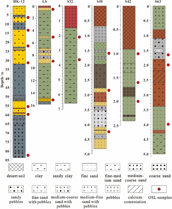
Figure S1
Lacustrine sedimentary profiles.
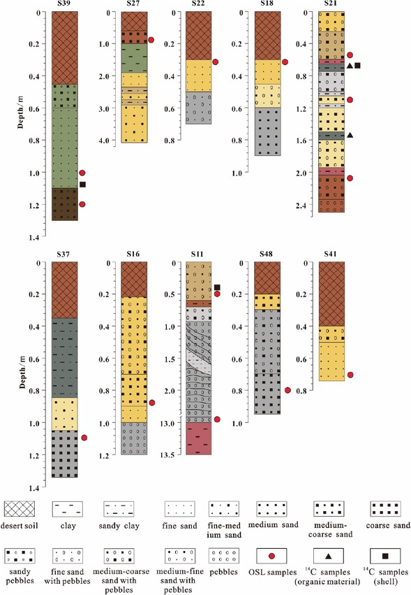
Figure S2
Lake shoreline profiles of the Jilantai Salt Lake.
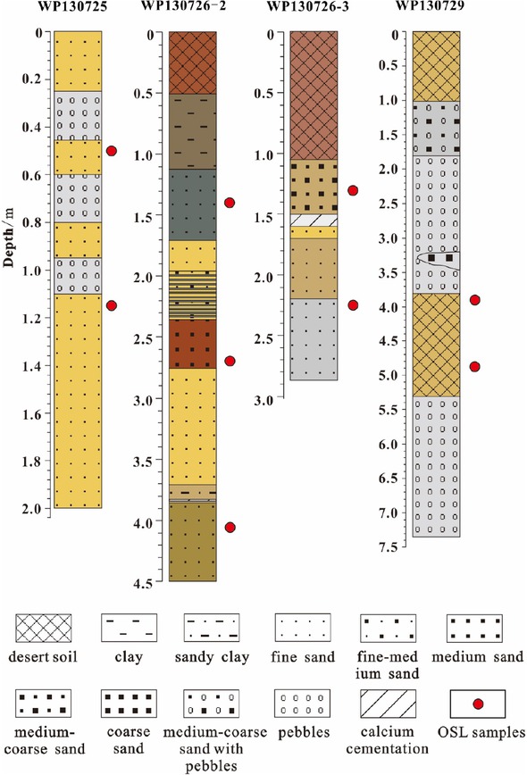
Figure S3
Fluvial sediment profiles.
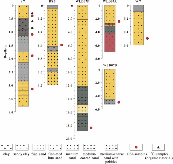
Figure S4
Desert sedimentary profiles.
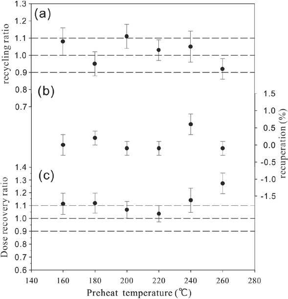
Figure S5
Results of a dose recovery test for a representative sample S63-2.
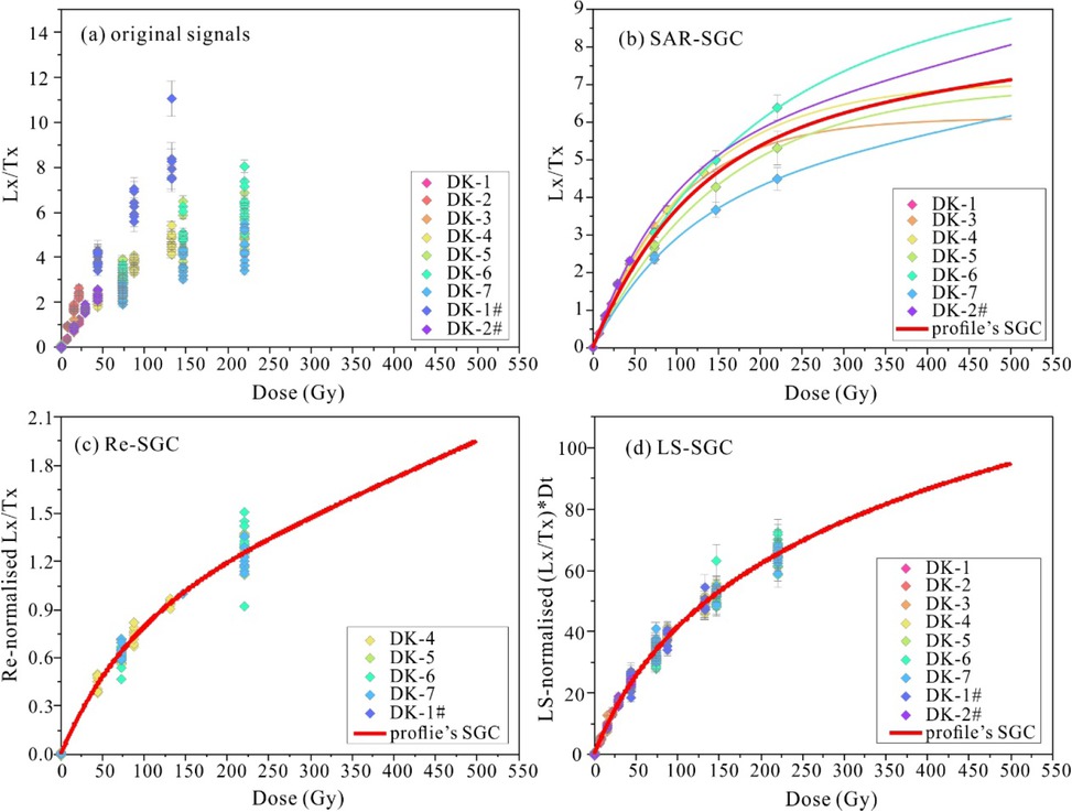
Figure S6
Comparison of SGCs for core DK12 established using three methods.
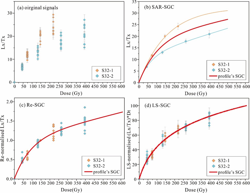
Figure S7
Comparison of SGCs for profile S32 established using three methods.
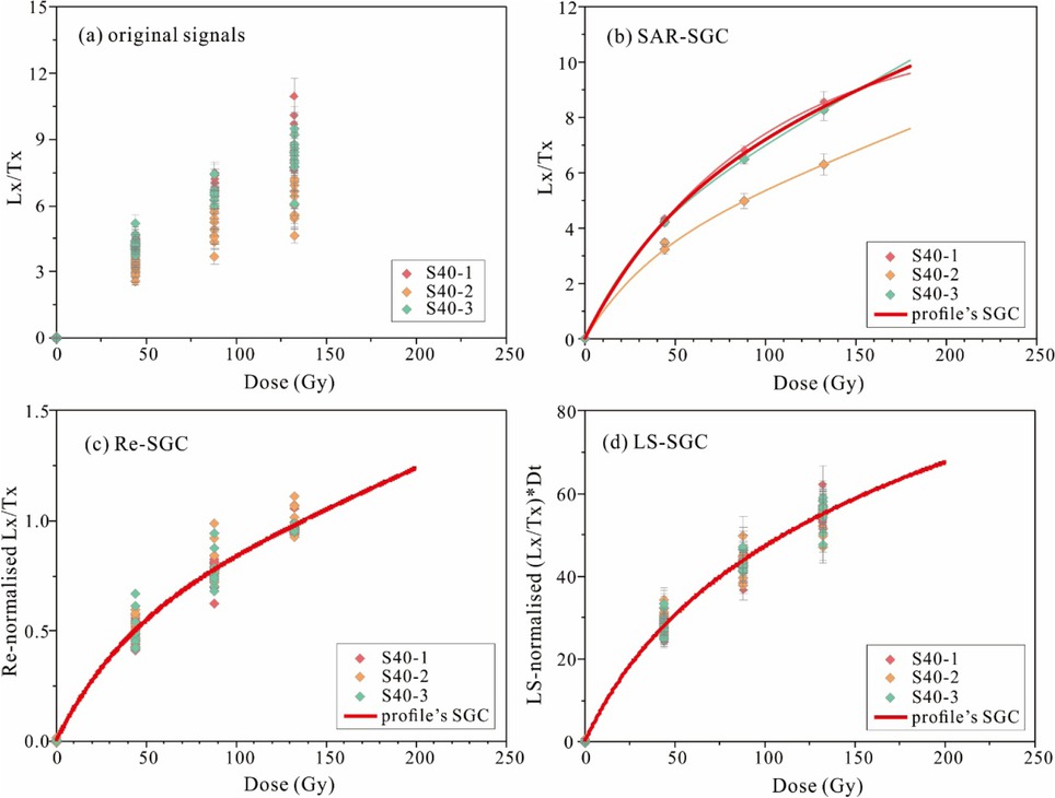
Figure S8
Comparison of SGCs for profile S40 established using three methods.
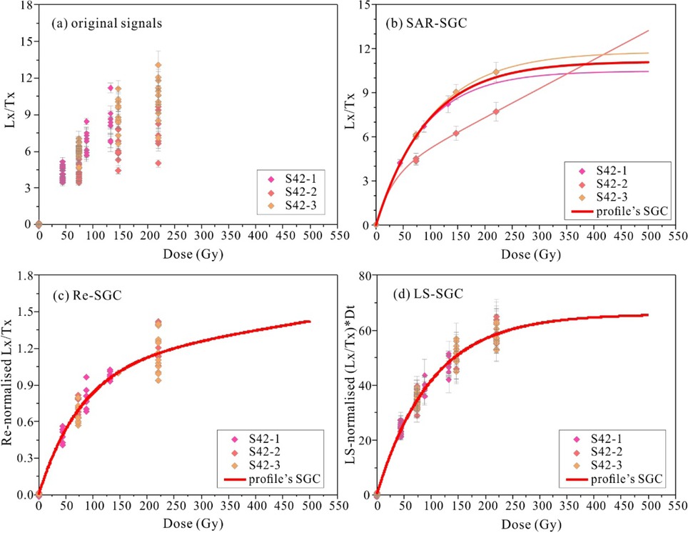
Figure S9
Comparison of SGCs for profile S42 established using three methods.
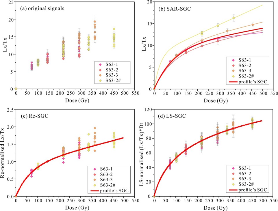
Figure S10
Comparison of SGCs for profile S63 profile established using three methods.
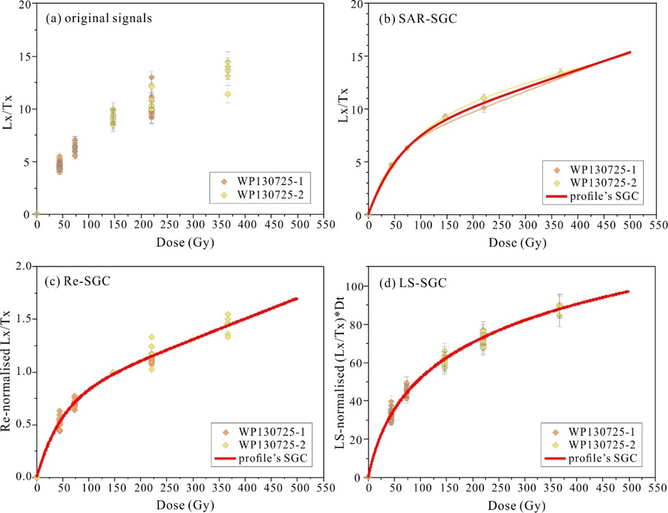
Figure S11
Comparison of SGCs for profile WP130725 established using three methods.
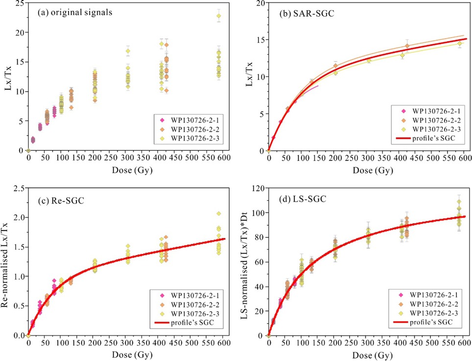
Figure S12
Comparison of SGCs for profile WP130726-2 established using three methods.
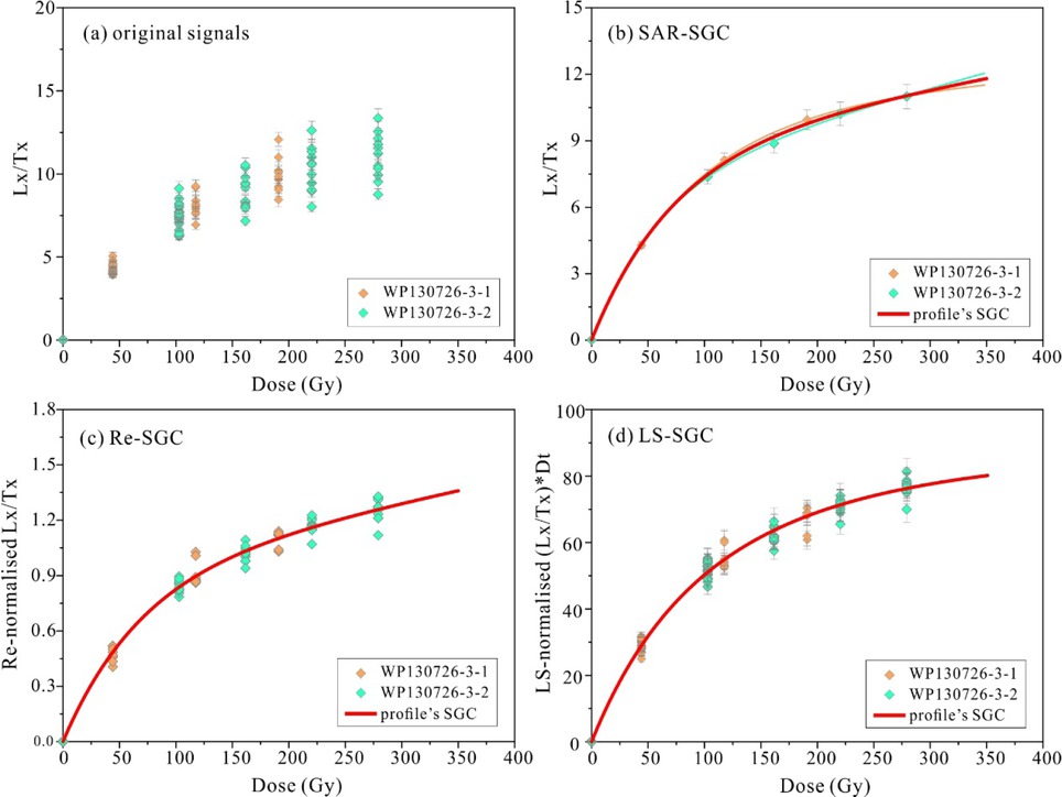
Figure S13
Comparison of SGCs for profile WP130726-3 established using three methods.
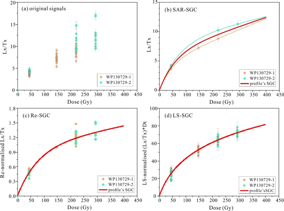
Figure S14
Comparison of SGCs for profile WP130729 established using three methods.