

Fig. 1
Procedure of fabric characterisation and defect detection
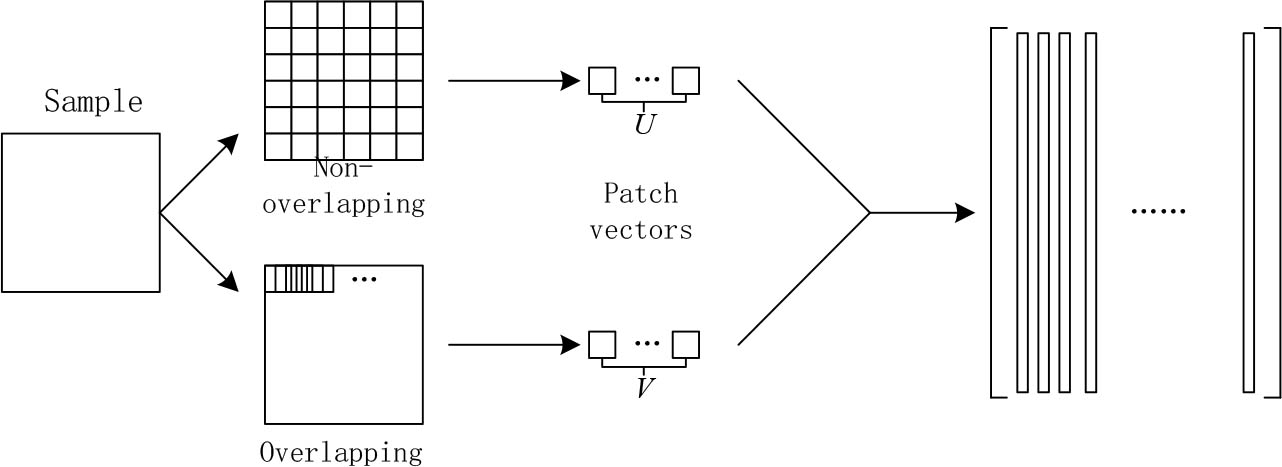
Fig. 2
Flow chart of a small patch partition

Fig. 3
Visual reconstruction samples with different dictionary sizes: (a) reconstruction of plain fabric image; (b) reconstruction of twill fabric image.
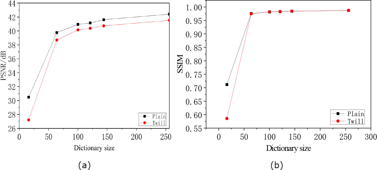
Fig. 4
Representation result of the fabric samples with different dictionary sizes k: (a) PSNR; (b) SSIM
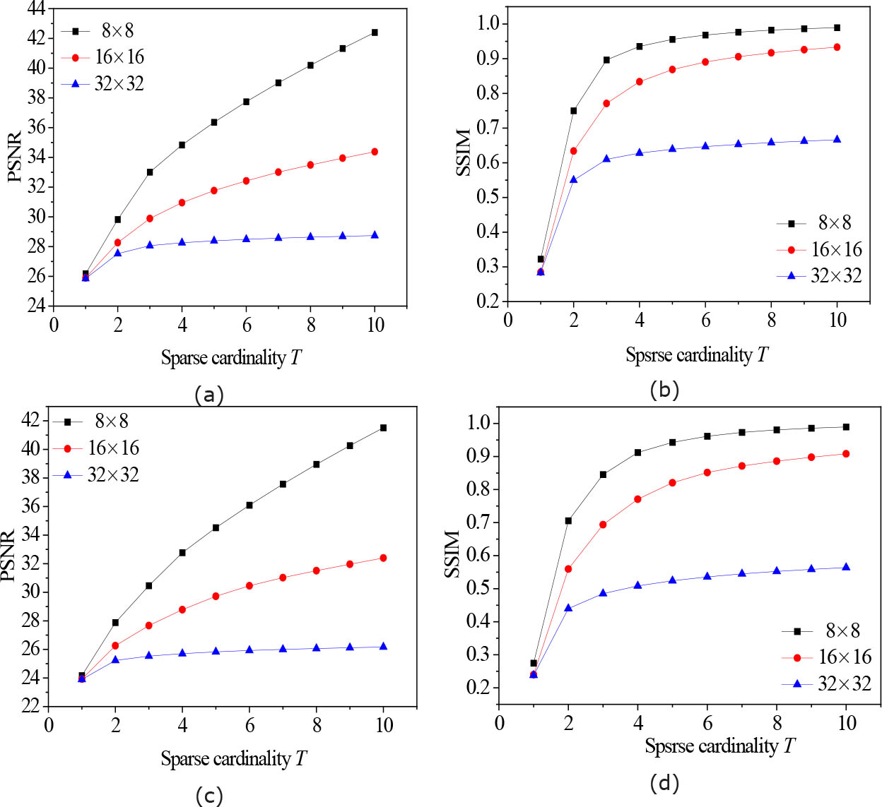
Fig. 5
Representation results for two fabric samples: (a) and (b) are plain fabric's PSNR and SSIM for different patch sizes with various sparse cardinality T; (c) and (d) are twill fabric's PSNR and SSIM for different patch sizes with various sparse cardinality T
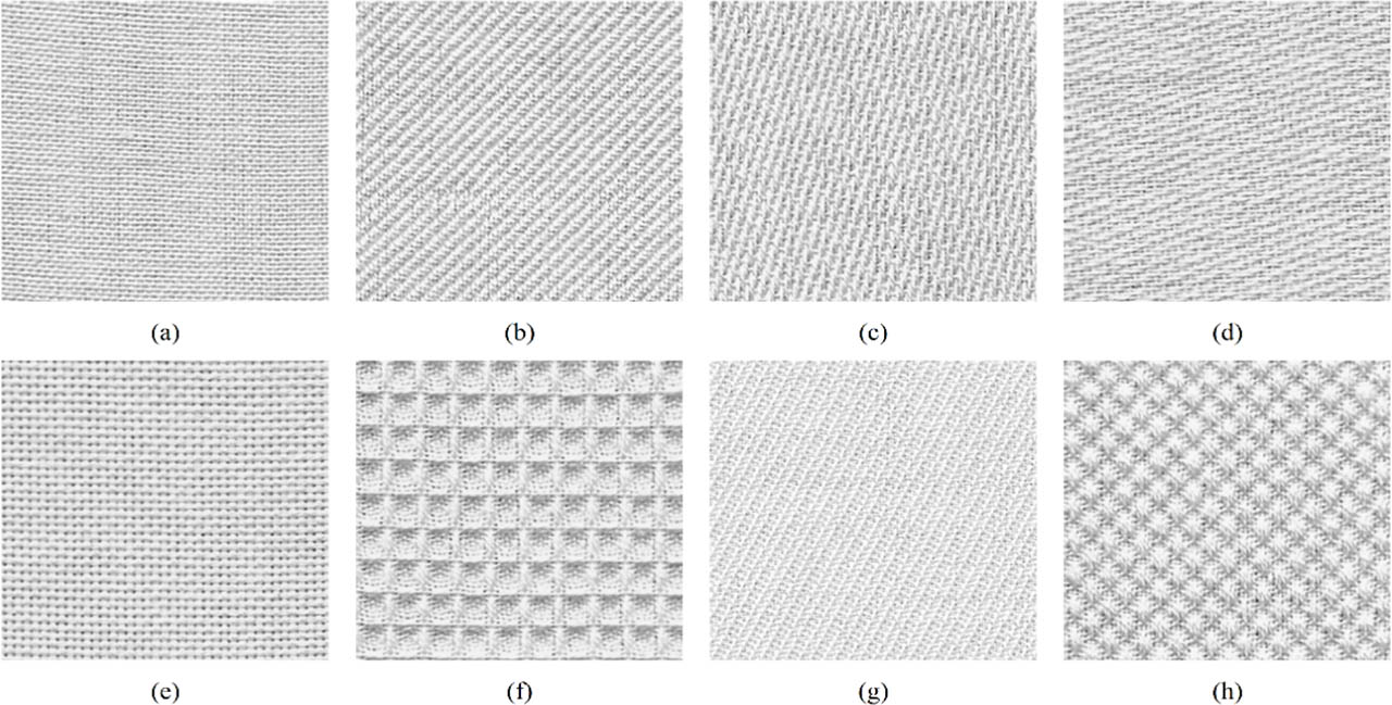
Fig. 6
Original fabric sample with different weave patterns: (a) plain, (b) twill, (c) weft satin,(d) warp satin, (e) basket weave, (f) honeycomb, (g) compound twill, (h) diamond twill
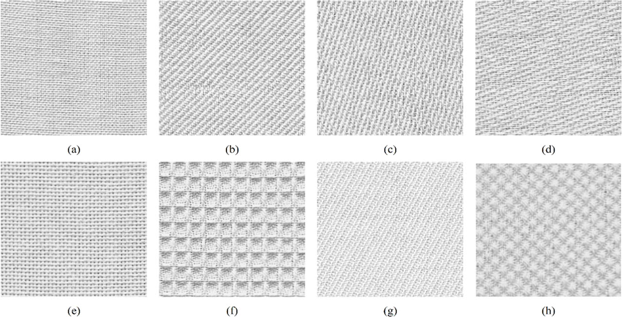
Fig. 7
Reconstructed fabric samples: (a) plain, (b) twill, (c) weft satin, (d) warp satin, (e) basket weave, (f) honeycomb, (g) compound twill, (h) diamond twill.
Table 1
Texture period for various weave patterns, for every weave pattern, the left is warp period and the right is weft period
| No. Sample | Plain | twill | warp satin | weft satin | basket weave | honey comb | compound twill | diamond twill | ||||||||
|---|---|---|---|---|---|---|---|---|---|---|---|---|---|---|---|---|
| 1 | 11 | 17 | 14 | 14 | 5 | 19 | 15 | 14 | 11 | 10 | 5 | 5 | 20 | 22 | 25 | 20 |
| 2 | 6 | 7 | 7 | 10 | 5 | 5 | 13 | 17 | 8 | 7 | 10 | 10 | 11 | 18 | 17 | 9 |
| 3 | 3 | 3 | 6 | 7 | 14 | 17 | 14 | 10 | 6 | 8 | 9 | 12 | 11 | 13 | 16 | 9 |
| 4 | 7 | 7 | 8 | 6 | 12 | 13 | 6 | 16 | 7 | 7 | 16 | 14 | 15 | 12 | 12 | 9 |
| 5 | 11 | 8 | 9 | 9 | 28 | 14 | 17 | 23 | 6 | 6 | 9 | 26 | 13 | 12 | 28 | 28 |
| Average | 8 | 8 | 9 | 9 | 13 | 14 | 13 | 16 | 8 | 8 | 10 | 13 | 14 | 15 | 20 | 15 |
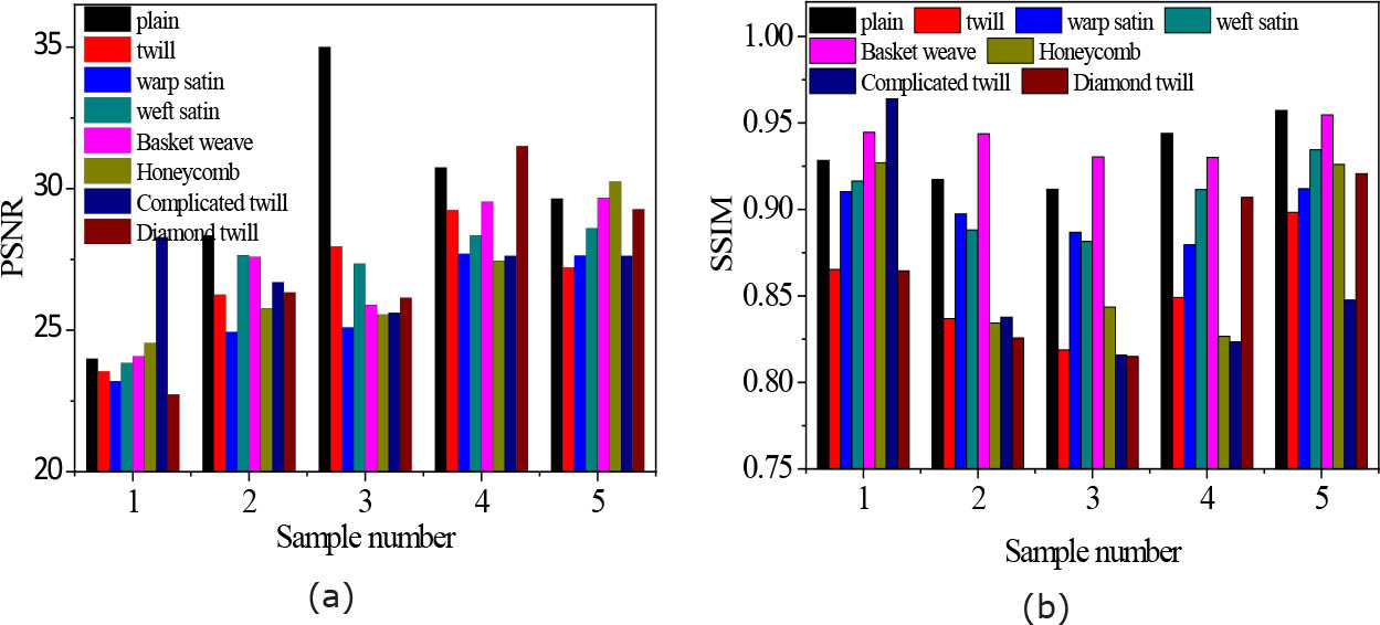
Fig. 8
Representation results of all test samples; (a) PSNR, (b) SSIM
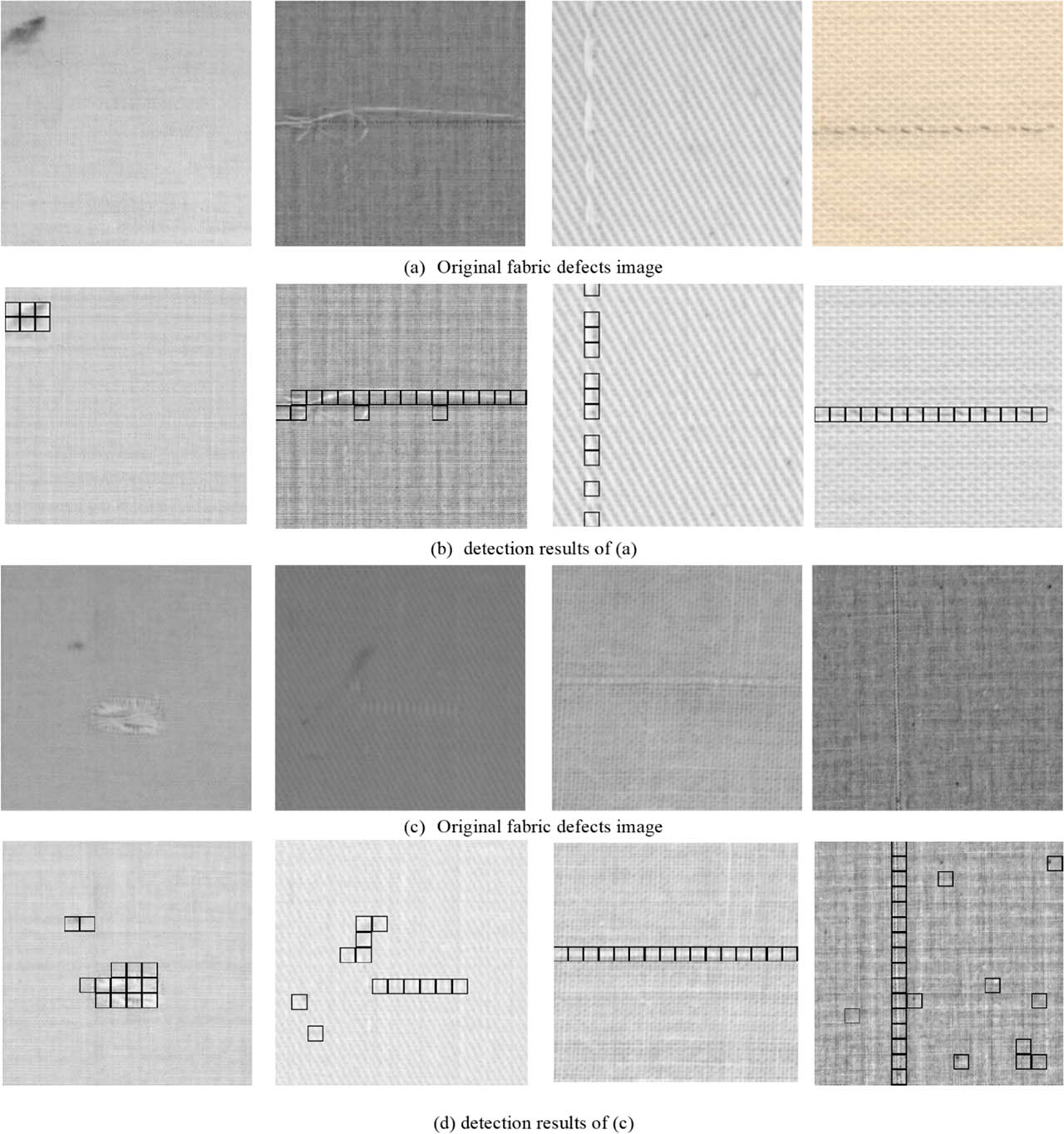
Fig. 9
Fabric defect detection result