
Table 1.
Summary of the parameters obtained from applying clustering algorithms to the strongest signal location within the SMEAR Estonia footprint. The averages and standard deviations of discrete variables have been rounded to the nearest integer. The execution time is measured in seconds per iteration.
| Scaler | DBSCAN | HDBSCAN | ||
|---|---|---|---|---|
| Standard | Robust | Standard | Robust | |
| ϵ | 0.48 ± 0.23 | 0.48 ± 0.23 | 0.26 ±0.14 | 0.23 ± 0.14 |
| minPts | 25 ± 14 | 25 ± 14 | 31 ± 12 | 31 ± 12 |
| Clusters (min. max) | 3 ± 10 (0. 285) | 2 ± 6 (0. 293) | 3 ± 1 (0. 25) | 3 ± 1 (0. 20) |
| Outliers | 169 ± 256 | 107 ± 202 | 224 ± 126 | 209 ± 132 |
| (min. max) | (0.1274) | (0. 1195) | (3. 938) | (3. 963) |
| Silhouette score | 0.31 ± 0.20 | 0.36 ±0.19 | 0.27 ± 0.14 | 0.30 ±0.15 |
| Davies-Bouldin score | 3.38 ± 6.99 | 3.35 ± 8.22 | 3.03 ±5.11 | 2.8 ± 1.6 |
| Execution time in s/it | 8.3 | 7.3 | 6.5 | 5.6 |
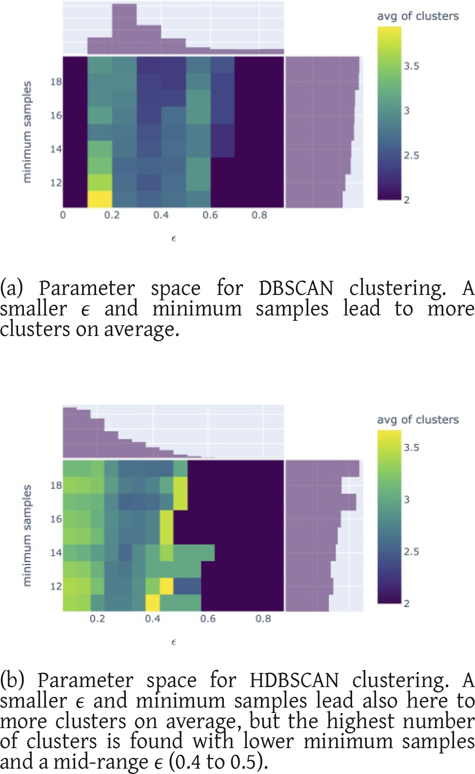
Figure 1.
We filtered the calculated results to match the number of clusters ranging between 2 and 6, a silhouette score above 0.3, the minimum samples (minPts) in the range of 10 to 20, and the Davies-Bouldin score below 3.5. Marginal distributions of the hyper-parameters are shown atop and right.
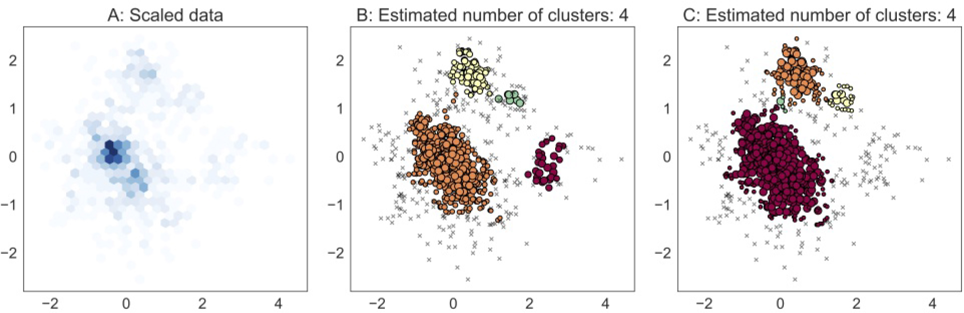
Figure 2.
Example of clusters detected among data for July 2015 with parameters ϵ = 0.3 and minPts = 15. Panel A shows the data scaled by the RobustScaler function and the color denotes the number of points per grid cell with a darker color for higher frequency. Panel B shows the estimated clusters using HDBSCAN, and C by DBSCAN. Note: The order in cluster labelling is different for the algorithms and therefore the coloring differs.
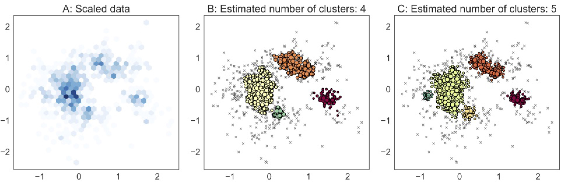
Figure 3.
Example of clusters detected among data for July 2017 with parameters ϵ = 0.15 and minPts = 17. The panels follow the logic given in Figure 2.