
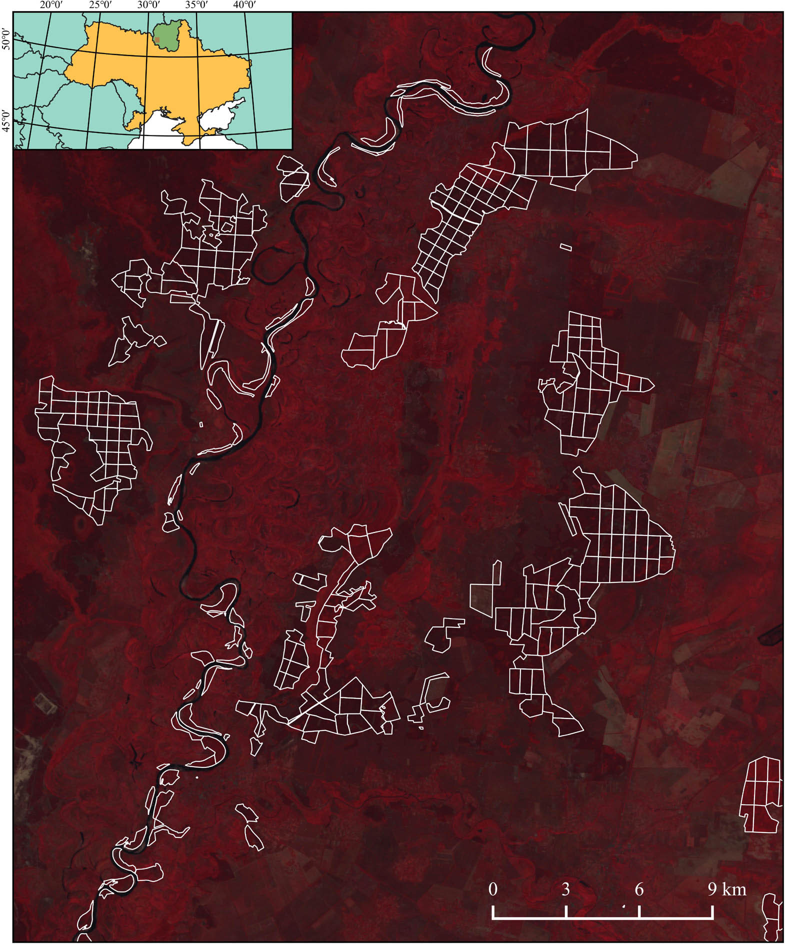
Figure 1
Location of the study site. The Chernihiv region (green) and study area (red) are coloured on the context map in the top. White lines refer to the edges of local forest management polygons used in this study, while the background is a raw Landsat image given in the band combination Near Infrared-Red-Green.
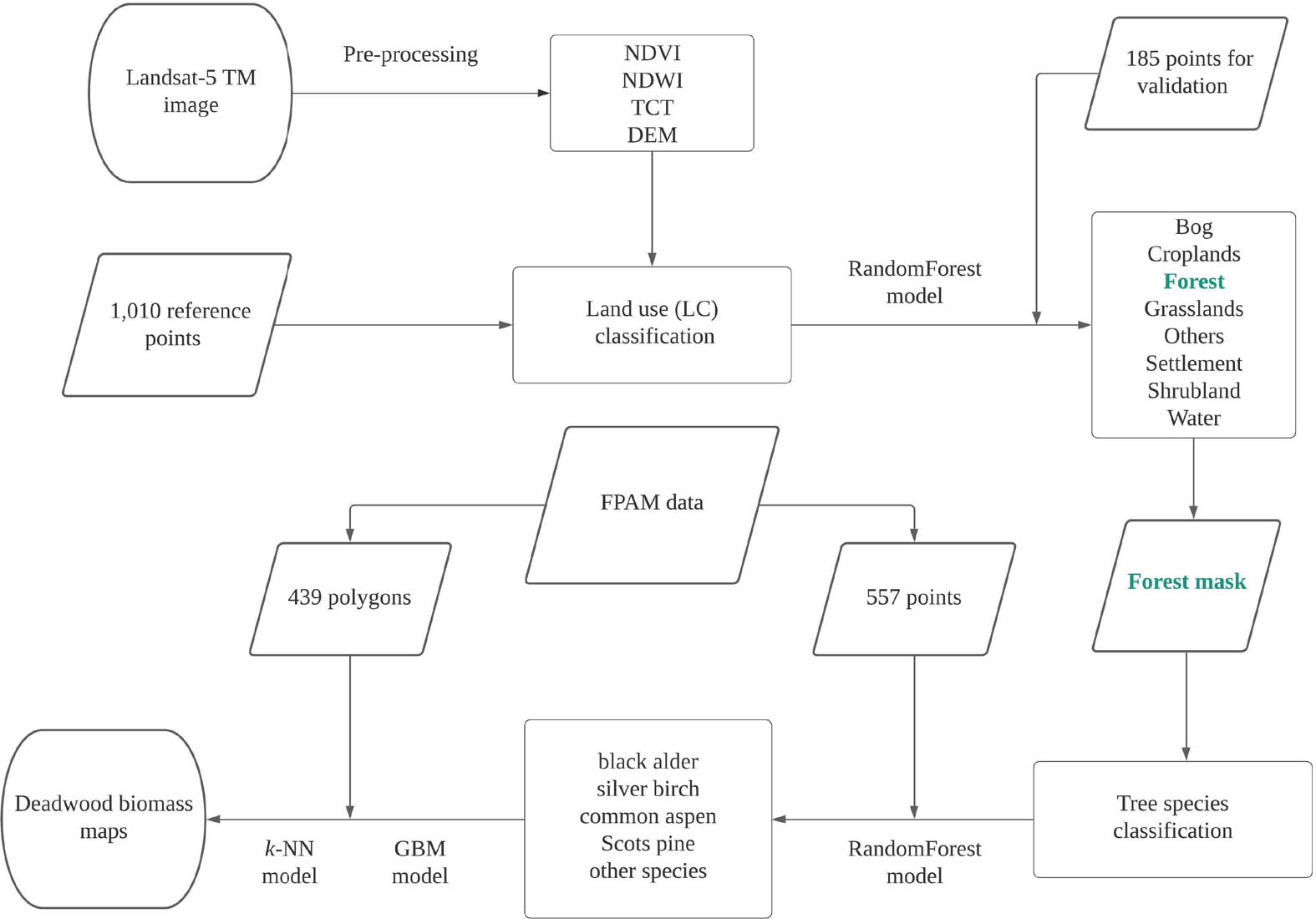
Figure 2
Workflow of the study. The flowchart illustrates utilization of the data, and the modelling process for classification and imputation purposes.
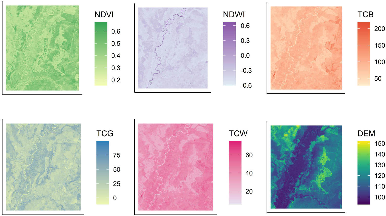
Figure 3
Ancillary datasets used for spatial modelling. The DEM variable is given in meters above sea level.
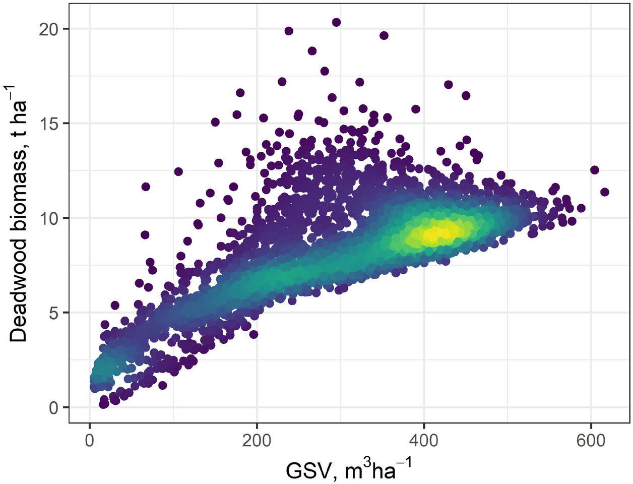
Figure 4
Scatterplot of the relationship between mean GSV and deadwood biomass stocks within the study area. Coloured gradient represents the density of points.
Table 1
Hyperparameter grid for tuning GBM models in this study.
| Parameter to tune | Hyperparameter values | |||||
|---|---|---|---|---|---|---|
| Shrinkage | 0.01 | 0.05 | 0.02 | 0.001 | ||
| Interaction depth | 2 | 4 | 6 | 8 | 10 | |
| Number of trees | 1000 | 5000 | 10000 | |||
| Number of observations in the terminal nodes | 5 | 10 | 15 | |||
| Bagging fraction | 0.5 | 0.75 | 1.0 | |||
Table 2
Confusion matrix of RF land cover classification.
| Predicted | Observed | |||||||
|---|---|---|---|---|---|---|---|---|
| Bog | Croplands | Forest | Grasslands | Others | Settlement | Shrubland | Water | |
| Bog | 13 | 0 | 1 | 0 | 0 | 0 | 1 | 0 |
| Croplands | 0 | 348 | 11 | 10 | 19 | 12 | 7 | 0 |
| Forest | 6 | 5 | 261 | 6 | 0 | 1 | 11 | 0 |
| Grasslands | 1 | 22 | 2 | 111 | 0 | 1 | 19 | 1 |
| Others | 0 | 0 | 0 | 0 | 0 | 1 | 0 | 0 |
| Settlement | 0 | 4 | 2 | 0 | 2 | 15 | 1 | 0 |
| Shrubland | 1 | 6 | 6 | 14 | 0 | 0 | 14 | 1 |
| Water | 1 | 0 | 0 | 0 | 0 | 0 | 0 | 27 |
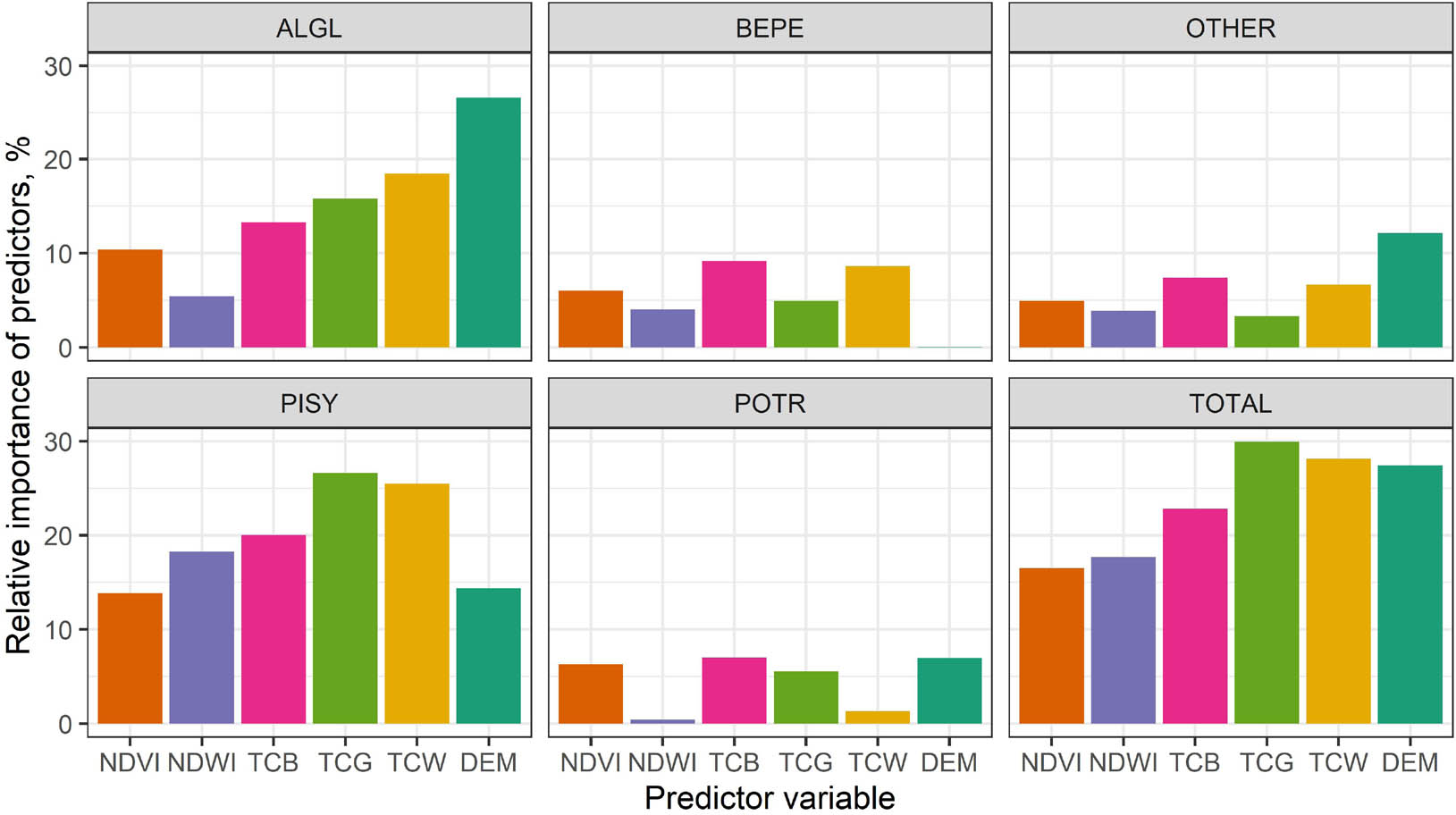
Figure 5
Importance of predictors for specific tree species and in total given by the RF classification model.
Table 3
Confusion matrix of RF tree species classification.
| Predicted | Observed | ||||
|---|---|---|---|---|---|
| ALGL | BEPE | OTHER | PISY | POTR | |
| ALGL | 12 | 1 | 5 | 4 | 3 |
| BEPE | 0 | 12 | 3 | 7 | 0 |
| OTHERS | 0 | 0 | 3 | 1 | 2 |
| PISY | 3 | 7 | 2 | 117 | 0 |
| POTR | 0 | 0 | 0 | 1 | 2 |
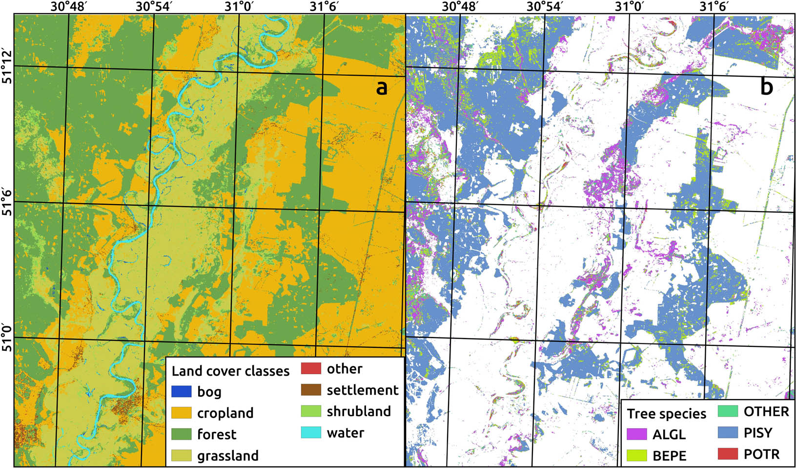
Figure 6
Land cover classes map (a) and tree species map within the forest mask (b) produced by the respective RF model.
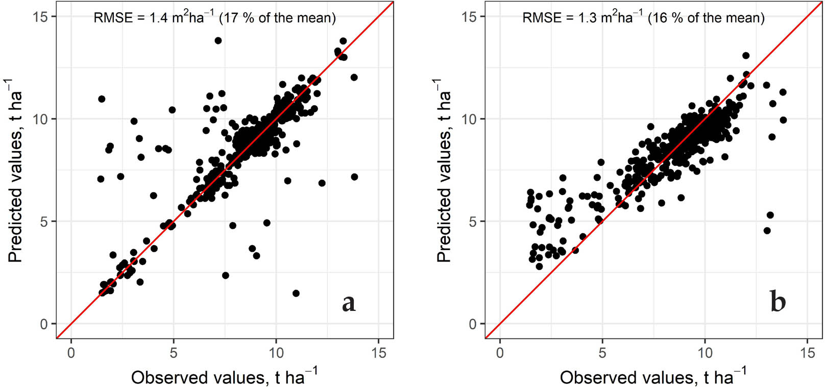
Figure 7
Agreement between predicted and observed values of deadwood biomass: imputed by the best k-NN (a, k = 1) and GBM (b) models.
Table 4
Comparison of mean and total values of deadwood biomass stock within the study area produced by the best performing models.
| Type of model | Tree species | ||||
|---|---|---|---|---|---|
| ALGL | BEPE | OTHER | PISY | POTR | |
| Mean ± SD, t·ha−1 | |||||
| k-NN | 7.0 ± 3.4 | 8.5 ± 1.9 | 8.1 ± 2.8 | 8.6 ± 1.9 | 8.1 ± 2.1 |
| GBM | 6.8 ± 2.3 | 8.0 ± 1.7 | 8.1 ± 1.7 | 8.4 ± 1.5 | 8.1 ± 2.1 |
| Total, thousands t | |||||
| k-NN | 39.0 | 34.8 | 19.9 | 237.6 | 4.9 |
| GBM | 37.9 | 32.8 | 19.9 | 232.0 | 4.9 |
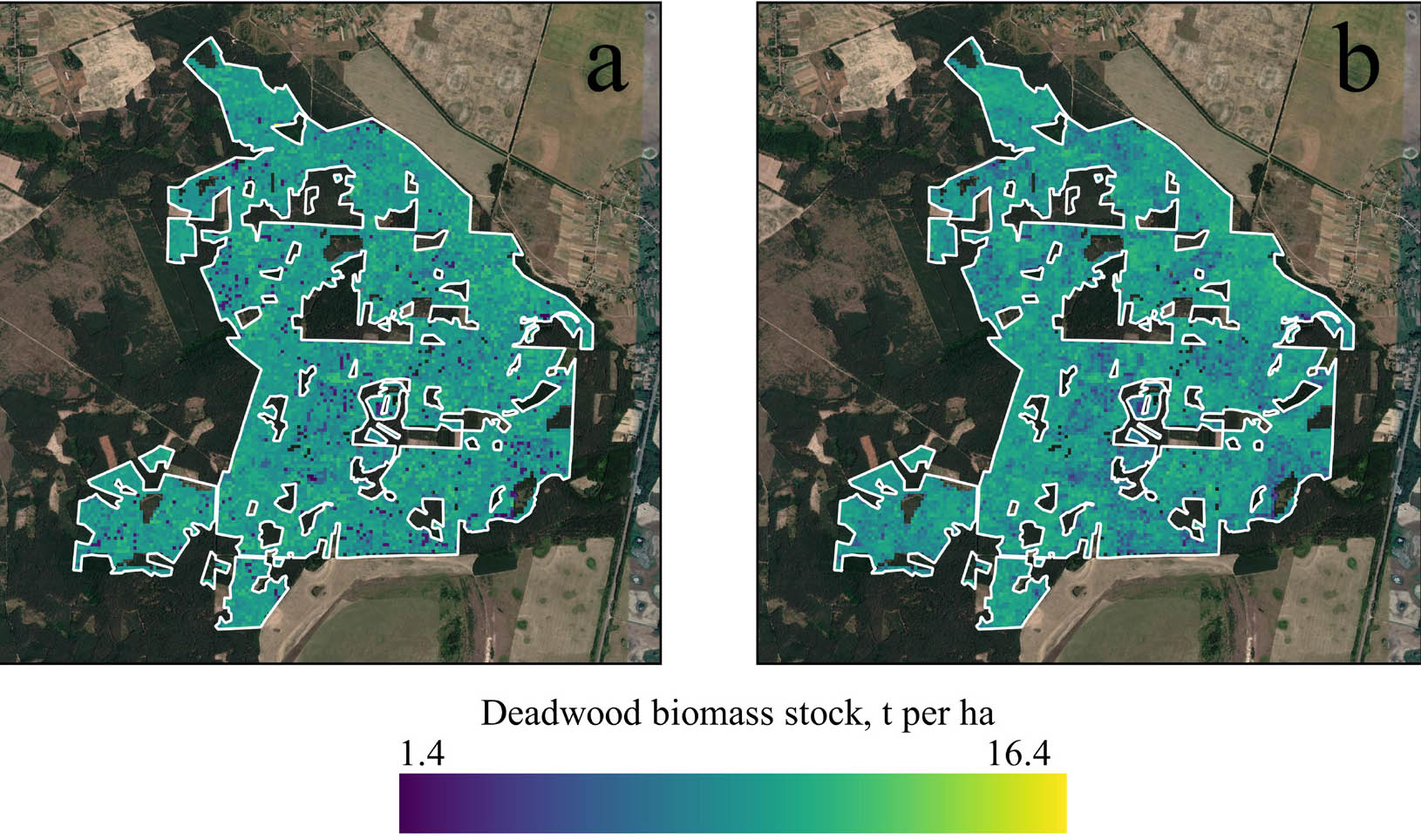
Figure 8
Test landscape with predicted deadwood biomass stock: imputed by the k-NN model (a) or estimated by the GBM model (b).
Table 5
Comparison of mean and total values of deadwood biomass stock for the test landscape at polygon level.
| Type of model | Mean ± CI, t·ha−1 | Total stock, t | Mean difference with reference per polygon, t·ha−1 |
|---|---|---|---|
| Reference | 7.8 ± 0.3 | 8011 | – |
| k-NN | 9.0 ± 0.1 | 9107 | +4.5 |
| GBM | 8.7 ± 0.1 | 8996 | +4.1 |
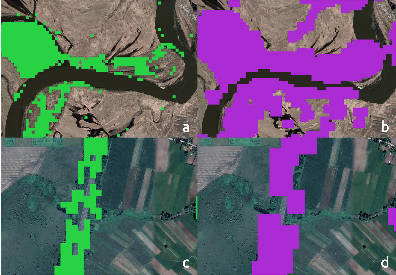
Figure 9
Subsets of predicted forest cover within the study area vs. actual linear stands across water bodies (a–b) and pathways (c–d). The green mask is produced by the RF model and the purple mask is created using GFC data.