

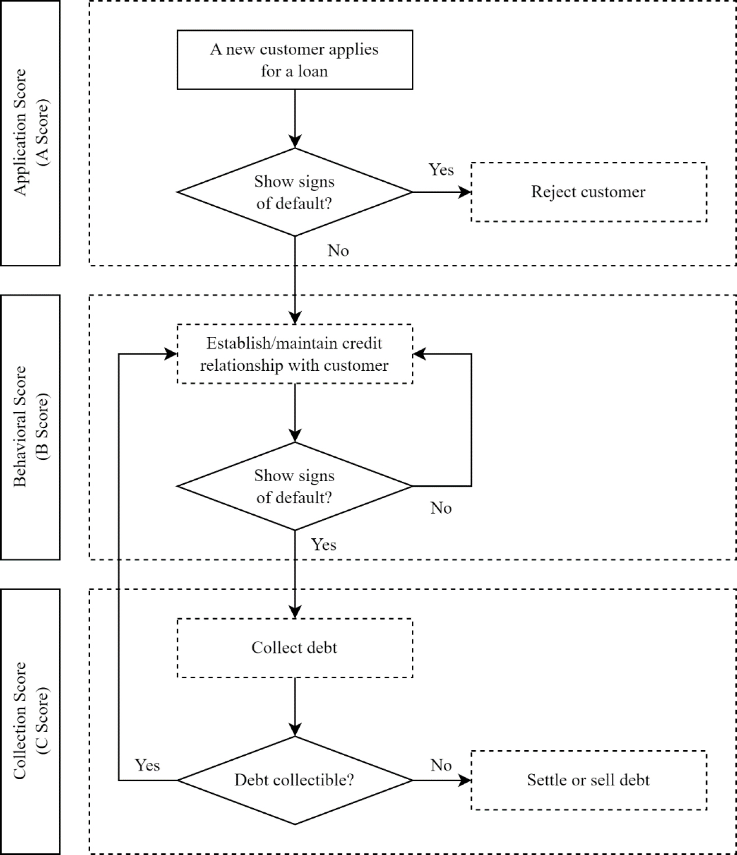
Figure 1.
The lifecycle of a customer’s credit relationship with a bank. (Source: Author’s own research)
Table 1.
Matrix for different types of alerts (Source: Reihart, et al., 2010)
| - | The event occurred | The event did not occur |
|---|---|---|
| There is a warning signal | A | B |
| There is no warning signal | C | D |
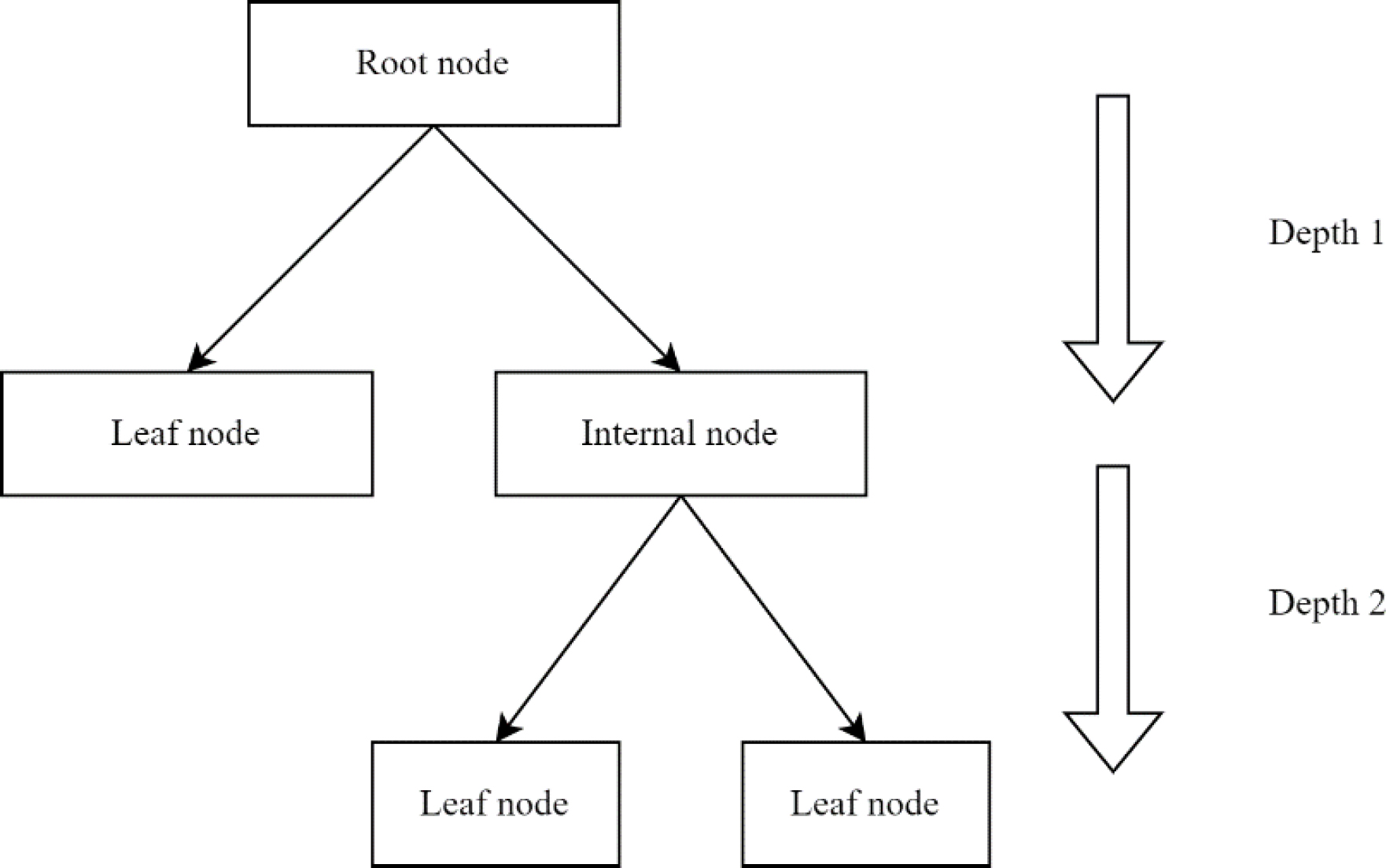
Figure 2.
A decision tree classifier (Source: Author’s illustration)
Table 2.
Summary of parameters of models (Source: Author’s compilation)
| Model | Parameter | Description |
|---|---|---|
| LG | None | The baseline model is a linear regression model combined with the sigmoid (logit) activation function, so no tuning is required |
| SVM | Kernel function | The activation function used to transform data into a different feature space for linear separation includes Linear, Polynomial, Sigmoid, and RBF |
| C | The coefficient for balancing the weight between distance and noise | |
| d | The degree parameter when using the Polynomial kernel, which takes a natural number value | |
| γ | The gamma parameter for Polynomial, Sigmoid, and RBF kernels, which takes a non-negative value | |
| r | The intercept for the Polynomial and Sigmoid kernels | |
| DT | Depth | It is necessary to limit the depth of the DT to avoid overfitting and reduce computational cost |
| Number of leaf nodes | It is necessary to limit the number of leaf nodes of the DT to avoid overfitting and reduce computational cost | |
| RF | Depth | It is necessary to limit the depth of each DT to avoid overfitting and reduce computational cost |
| Number of leaf nodes | It is necessary to limit the number of leaf nodes of each DT to avoid overfitting and reduce computational cost | |
| Number of DTs | The number of DTs in Random Forest Classifier (RF) needs to be considered for computational cost when the number is too high |
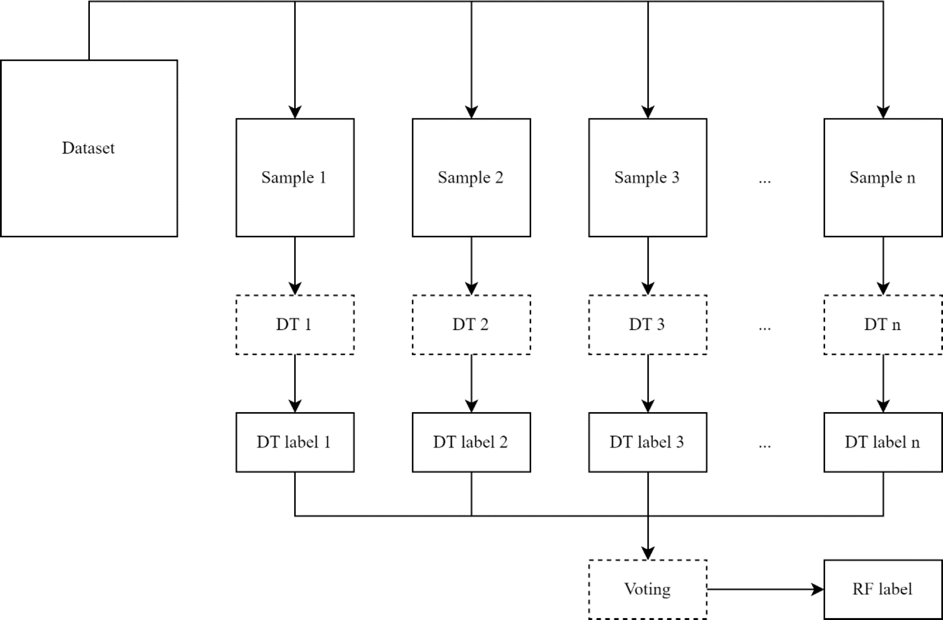
Figure 3.
A random forest classifier (Source: Author’s illustration)
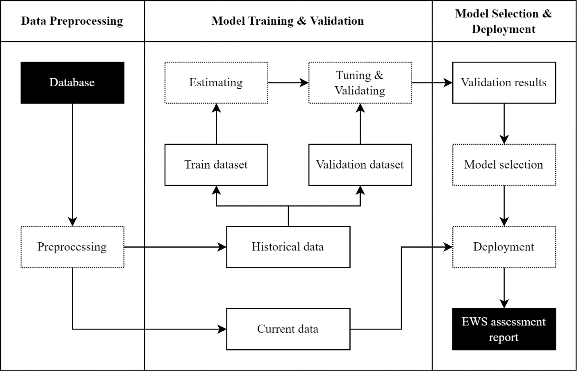
Figure 4.
A random forest classifier (Source: Author’s own research)
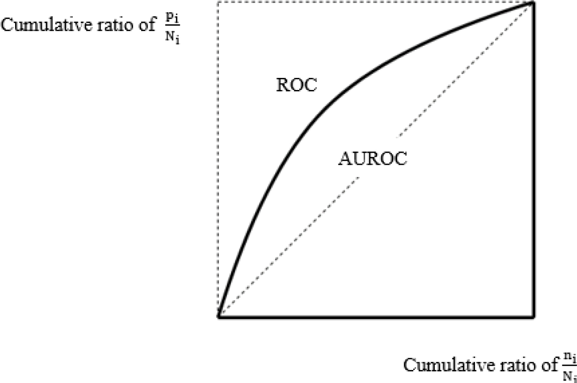
Figure 5.
ROC and AUROC (Source: Author’s illustration)
Table 3.
Model tuning parameters in Scikit-learn (Source: Author’s own research)
| Model | Parameter | Parameters in Scikit-learn | Range of values for tuning |
|---|---|---|---|
| LG | None | None | None |
| SVM | Kernel function | kernel: accepts a value from ‘linear’, ‘poly’, ‘rbf’, ‘sigmoid’. The default value is ‘rbf’ | ‘linear’, ‘poly’, ‘rbf’, ‘sigmoid’ |
| C | C: data type is float; the default value is 1 | 0.01, 0.1, 1, 10 | |
| d | degree: data type is integer; the default value is 3 | 2, 3, 4, 5 (this is applicable only when kernel is set to ‘poly’) | |
| γ | Gamma: accepts a value from ‘scale’, ‘auto’. The default value is ‘scale’. It can also be specified as a non-negative float | 0.01, 0.1, 1, 10 (not applicable when kernel is set to ‘linear’) | |
| DT | Depth | max_depth: data type is integer or none. The default value is none, which means the tree is expanded until the maximum depth is reached | The range from 2 to 21 (with a step size of 2) and none |
| Number of leaf nodes | max_leaf_nodes: data type is integer or None. The default value is none, which means an unlimited number of leaf nodes will be developed, regardless of max_depth | The range from 2 to 21 (with a step size of 2) and none | |
| RF | Depth | Similar to DT | Similar to DT |
| Number of leaf nodes | Similar to DT | Similar to DT | |
| Number of DTs | n_estimators, data type is integer. The default value is 100 | 10, 50, 100 |
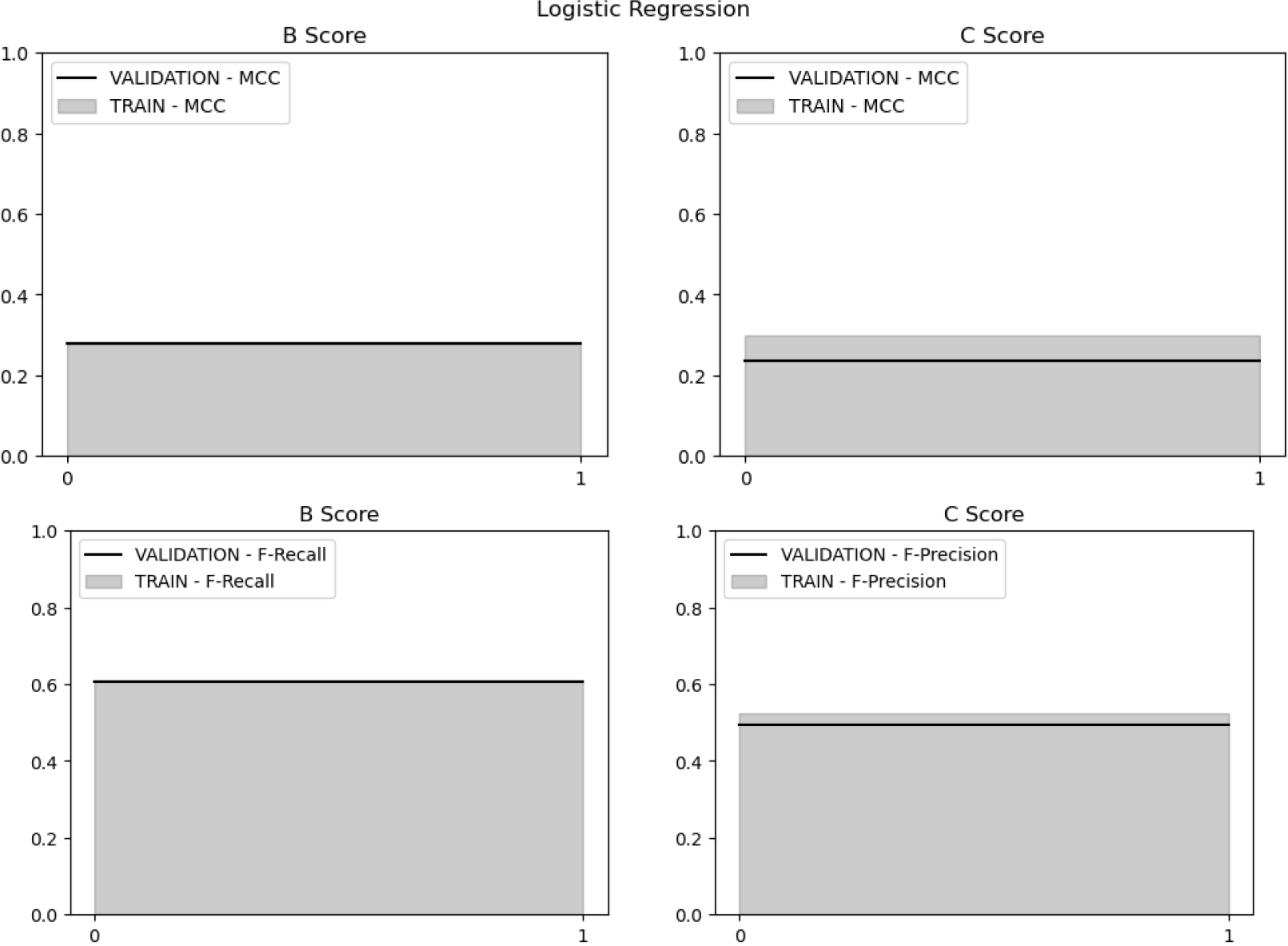
Figure 6.
Logistic regression results (Source: Author’s own calculation)
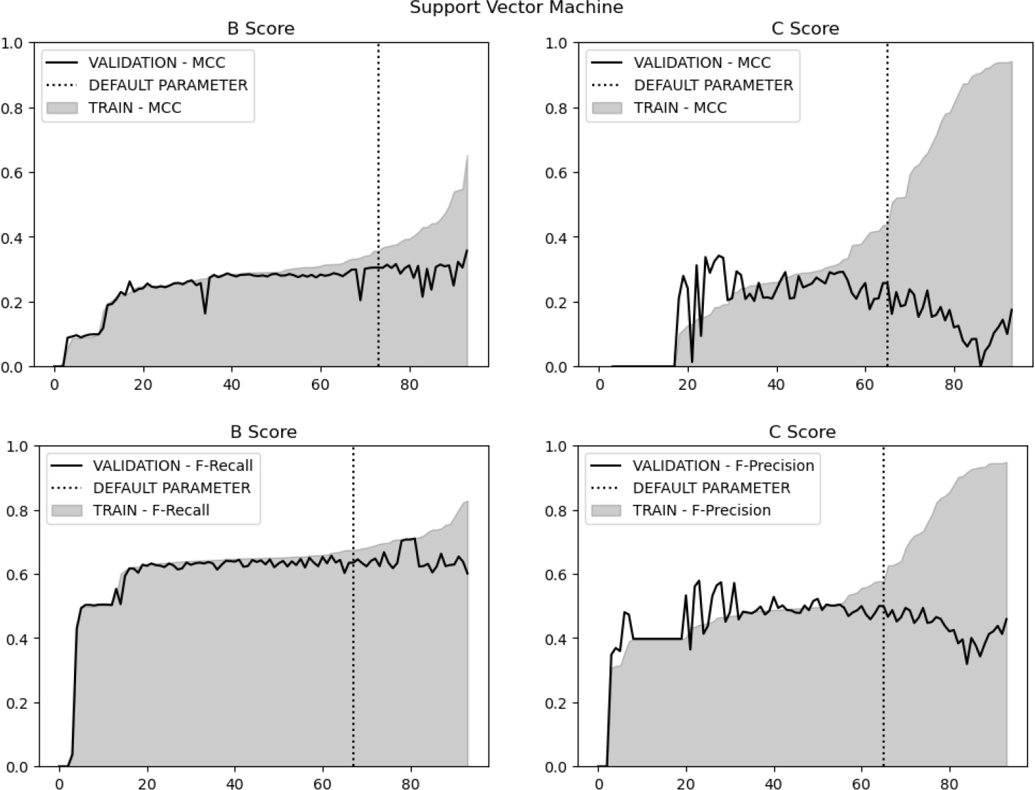
Figure 7.
Support vector machine results (Source: Author’s own calculation)
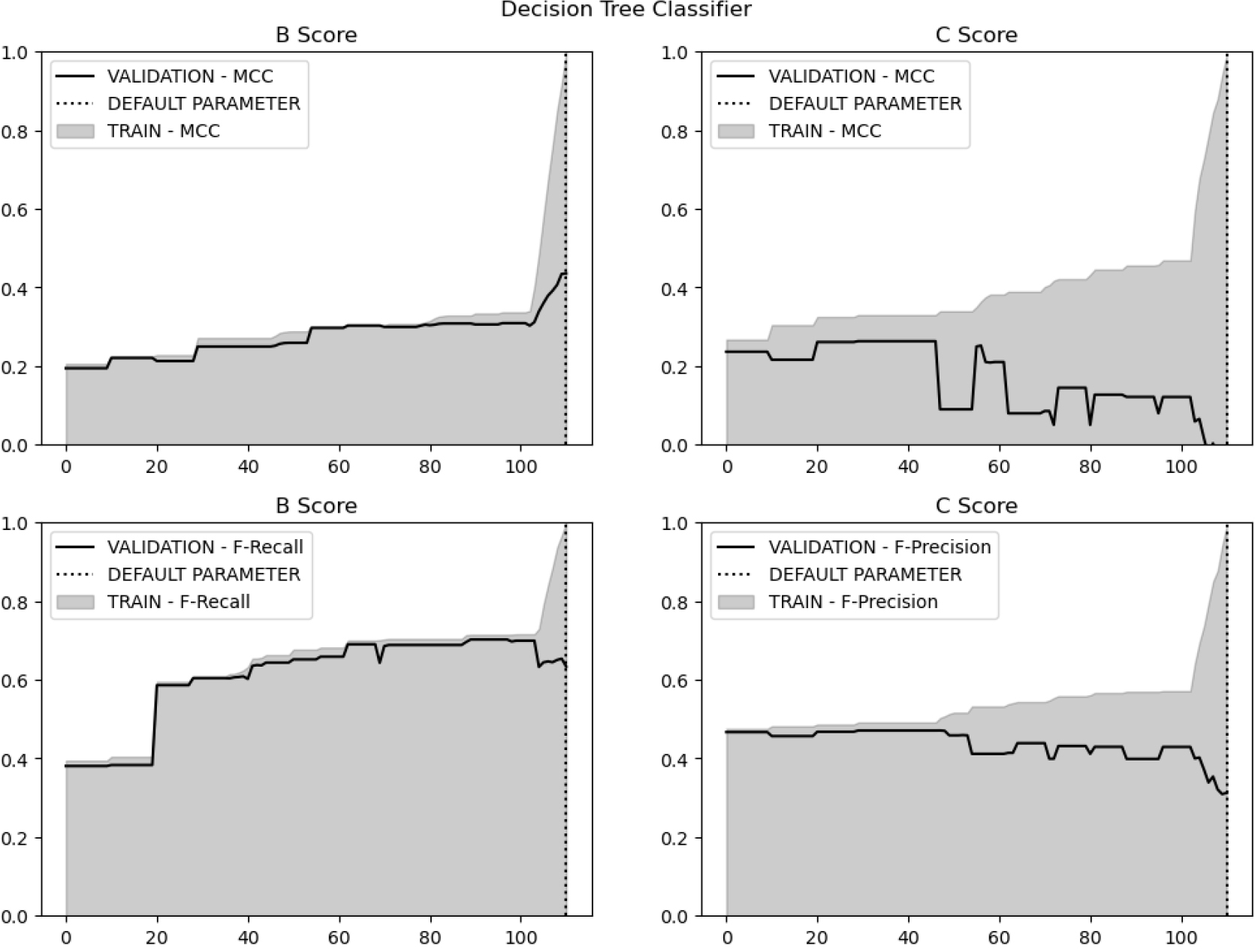
Figure 8.
Decision tree results. (Source: Author’s own calculation)
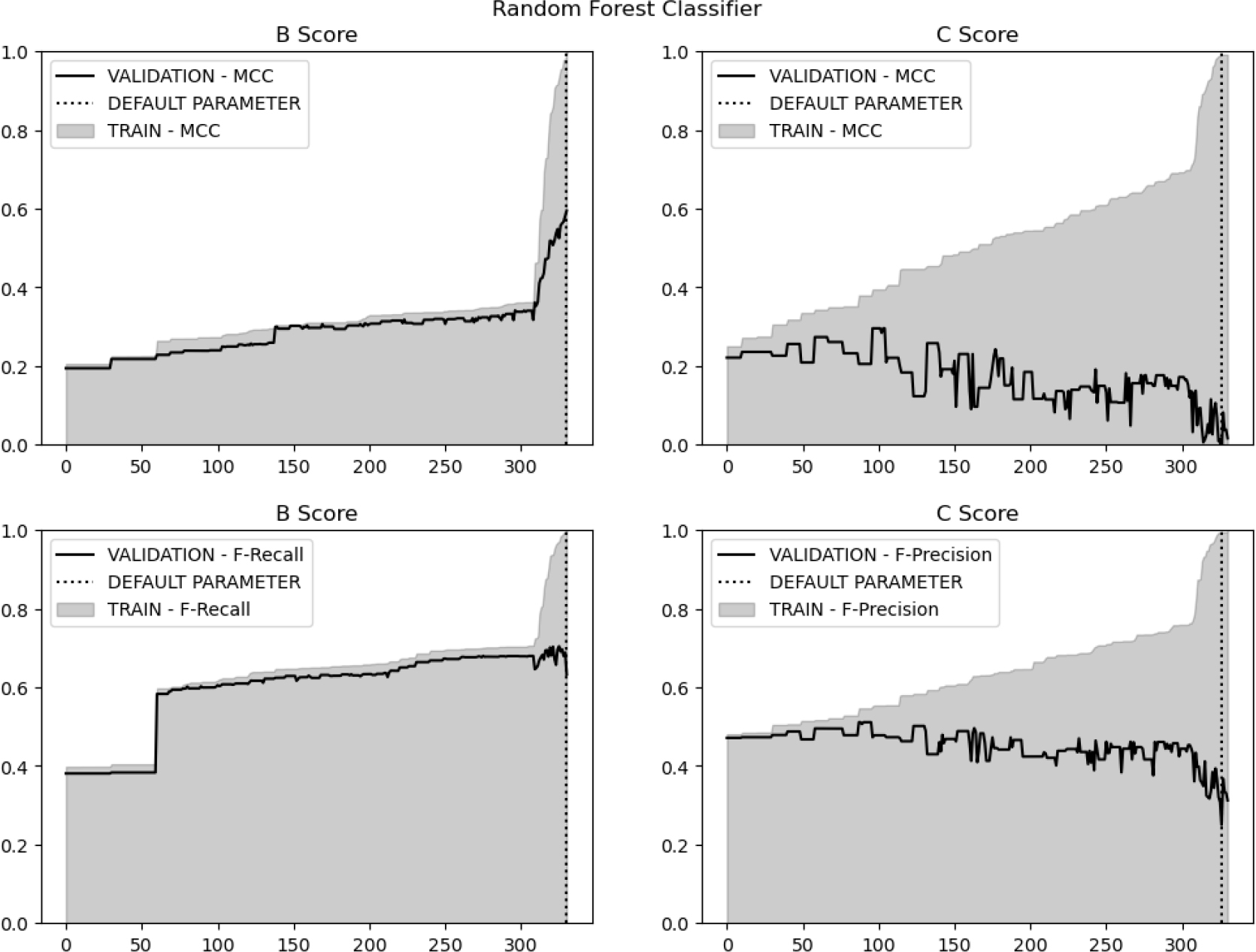
Figure 9.
Decision tree results (Source: Author’s own calculation)
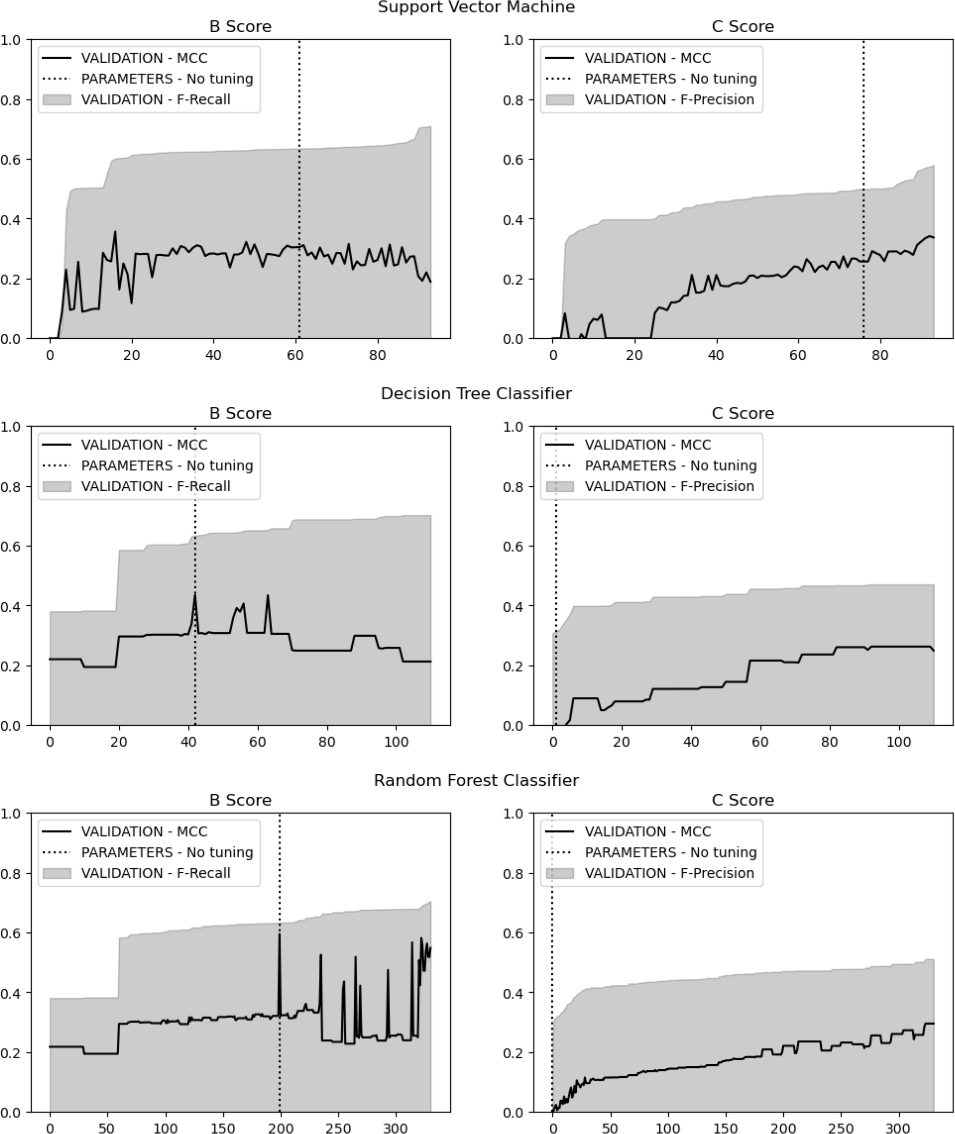
Figure 10.
MCC versus F-Recall and F-Precision (Source: Author’s own calculation)
Table 5.
The results of the evaluation criteria for the B Score model (Source: Author’s own calculation)
| Dataset | Criteria (%) | Tuned by MCC | Tuned by F-Recall | ||||||
| LR | SVM | DT | RF | LR | SVM | DT | RF | ||
| Train | Accuracy | 64.62 | 83.22 | 96.29 | 99.06 | 64.62 | 47.05 | 50.31 | 96.11 |
| Recall | 65.19 | 86.98 | 98.20 | 99.97 | 65.19 | 91.53 | 90.05 | 99.10 | |
| Precision | 47.59 | 69.86 | 91.29 | 97.27 | 47.59 | 37.73 | 39.19 | 90.15 | |
| F1 | 55.02 | 77.48 | 94.62 | 98.60 | 55.02 | 53.44 | 54.61 | 94.41 | |
| F-Recall | 60.70 | 82.91 | 96.74 | 99.42 | 60.70 | 71.22 | 71.49 | 97.17 | |
| F-Precision | 50.31 | 72.72 | 92.59 | 97.80 | 50.31 | 42.76 | 44.18 | 91.81 | |
| MCC | 27.92 | 65.34 | 91.94 | 97.92 | 27.92 | 19.60 | 22.82 | 91.68 | |
| Validation | Accuracy | 64.66 | 70.58 | 74.09 | 81.84 | 64.66 | 46.62 | 50.41 | 79.85 |
| Recall | 64.98 | 61.58 | 66.95 | 67.45 | 64.98 | 91.48 | 87.83 | 70.78 | |
| Precision | 47.62 | 55.08 | 59.79 | 75.26 | 47.62 | 37.52 | 39.02 | 69.20 | |
| F1 | 54.96 | 58.15 | 63.17 | 71.14 | 54.96 | 53.22 | 54.04 | 69.98 | |
| F-Recall | 60.56 | 60.16 | 65.39 | 68.88 | 60.56 | 71.04 | 70.26 | 70.46 | |
| F-Precision | 50.31 | 56.27 | 61.10 | 73.56 | 50.31 | 42.54 | 43.90 | 69.51 | |
| MCC | 27.89 | 35.71 | 43.45 | 58.13 | 27.89 | 18.94 | 21.29 | 54.83 | |
Table 6.
The results of the evaluation criteria for the C Score model (Source: Author’s own calculation)
| Dataset | Criteria (%) | Tuned by MCC | Tuned by F-Precision | ||||||
| LR | SVM | DT | RF | LR | SVM | DT | RF | ||
| Train | Accuracy | 65.02 | 63.60 | 56.71 | 65.72 | 65.02 | 63.60 | 58.66 | 65.72 |
| Recall | 67.69 | 44.62 | 93.33 | 85.64 | 67.69 | 36.92 | 92.82 | 85.64 | |
| Precision | 49.44 | 47.03 | 43.96 | 50.15 | 49.44 | 46.45 | 45.14 | 50.15 | |
| F1 | 57.14 | 45.79 | 59.77 | 63.26 | 57.14 | 41.14 | 60.74 | 63.26 | |
| F-Recall | 63.04 | 45.08 | 76.21 | 75.02 | 63.04 | 38.50 | 76.63 | 75.02 | |
| F-Precision | 52.26 | 46.52 | 49.16 | 54.68 | 52.26 | 44.17 | 50.31 | 54.68 | |
| MCC | 29.80 | 18.44 | 33.02 | 39.49 | 29.80 | 15.51 | 35.05 | 39.49 | |
| Validation | Accuracy | 63.79 | 70.78 | 53.91 | 62.55 | 63.79 | 71.60 | 54.73 | 62.55 |
| Recall | 57.14 | 53.57 | 89.29 | 75.00 | 57.14 | 45.24 | 85.71 | 75.00 | |
| Precision | 48.00 | 58.44 | 42.13 | 47.37 | 48.00 | 62.30 | 42.35 | 47.37 | |
| F1 | 52.17 | 55.90 | 57.25 | 58.06 | 52.17 | 52.41 | 56.69 | 58.06 | |
| F-Recall | 55.05 | 54.48 | 72.96 | 67.16 | 55.05 | 47.86 | 71.15 | 67.16 | |
| F-Precision | 49.59 | 57.40 | 47.11 | 51.14 | 49.59 | 57.93 | 47.12 | 51.14 | |
| MCC | 23.62 | 34.19 | 26.33 | 29.60 | 23.62 | 33.75 | 24.98 | 29.60 | |
Table 7.
The results of the evaluation criteria for the C Score model (Source: Author’s own calculation)
| Customer | Model | Selection | Parameters |
|---|---|---|---|
| B Score | Best | RF tuned by MCC | n_estimators = 100; max_depth = 20; max_leaf_node = None |
| SVM tuned by F-Recall | kernel = ‘sigmoid’; C = 0.1; gamma = 0.01 | ||
| Second best | RF tuned by F-Recall | n_estimators = 100; max_depth = 16; max_leaf_node = None | |
| C Score | Best | SVM tuned by MCC | kernel = ‘poly’; degree = 4; C = 0.01 gamma = 0.1 |
| SVM tuned by F-Precision | kernel = ‘poly’; degree = 4; C = 0.1 gamma = 0.01 |
Table 8.
Early warning system deployment for B Score customers (Source: Author’s own calculation)
| Criteria (%) | Tuned by MCC | Tuned by F-Recall | |
|---|---|---|---|
| RF (best) | SVM (best) | RF (second best) | |
| Accuracy | 81.84 → 78.67 | 46.62 → 36.86 | 79.85 → 76.56 |
| Recall | 67.45 → 29.01 | 91.48 → 91.53 | 70.78 → 38.14 |
| Precision | 75.26 → 42.84 | 37.52 → 22.44 | 69.20 → 39.37 |
| F-Recall | 68.88 → 31.01 | 71.04 → 56.65 | 70.46 → 38.38 |
Table 9.
Early warning system deployment for C Score customers (Source: Author’s own calculation)
| Criteria (%) | Tuned by MCC | Tuned by F-Precision |
|---|---|---|
| SVM (best) | SVM (best) | |
| Accuracy | 70.78 → 61.94 | 71.60 → 65.54 |
| Recall | 53.57 → 54.48 | 45.24 → 50.00 |
| Precision (*) | 58.44 → 40.33 | 62.30 → 43.79 |
| F-Precision (*) | 57.40 → 42.54 | 57.93 → 44.91 |