
Table 1
Spraying dates within Experiments 1 and 2.
| Experiment type | Treatment | Dates | ||||||||
|---|---|---|---|---|---|---|---|---|---|---|
| 11th Feb | 18th Feb | 25th Feb | 3rd Mar | 10th Mar | 17th Mar | 24th Mar | 31st Mar | 7th Apr | ||
| 1 | Contr | Yes | Yes | Yes | Yes | Yes | Yes | |||
| Pf × Ab | Yes | Yes | Yes | Yes | Yes | Yes | ||||
| Pc | Yes | Yes | Yes | Yes | Yes | Yes | ||||
| Eth | Yes | Yes | Yes | Yes | Yes | Yes | ||||
| Mes | Yes | No | Yes | No | No | No | ||||
| 2 | Contr | Yes | Yes | Yes | Yes | Yes | Yes | |||
| Pf × Ab | Yes | Yes | Yes | Yes | Yes | Yes | ||||
| Pc | Yes | Yes | Yes | Yes | Yes | Yes | ||||
| Eth | Yes | Yes | Yes | Yes | Yes | Yes | ||||
| Mes | Yes | No | Yes | No | No | No | ||||
[i] Yes – spraying was performed; No – without spraying; Feb – February; Mar – March; Apr – April.
[ii] Eth, ethephon; Mes, mesotrione; Pc, prohexadione calcium.
Table 2
Repeated measures ANOVA parameters for the main effects and associated interaction for average plant height.
| Source between variables | df | F | p |
|---|---|---|---|
| All between | 30 | 41.13 | <0.05 |
| Intercept | 1 | 33.12 | <0.05 |
| Treatment | 4 | 61.34 | <0.05 |
| Turfgrass species | 2 | 42.72 | <0.05 |
| Experiment type | 1 | 14.23 | <0.05 |
| Treatment × turfgrass species | 8 | 8.10 | <0.05 |
| Treatment × experiment type | 4 | 0.66 | 0.053 |
| Turfgrass species × experiment type | 2 | 8.26 | <0.05 |
| Treatment × turfgrass species × experiment type | 8 | 2.03 | <0.05 |
| Source within Experiment 1 | |||
| Within interactions | 140 | 87.12 | <0.05 |
| Date of evaluation | 18 | 1,749.17 | <0.05 |
| Treatment | 4 | 154.24 | <0.05 |
| Turfgrass species | 2 | 197.68 | <0.05 |
| Date of evaluation × treatment | 72 | 29.46 | <0.05 |
| Date of evaluation × turfgrass species | 36 | 122.71 | <0.05 |
| Treatment × turfgrass species | 8 | 132.78 | <0.05 |
| Source within Experiment 2 | |||
| Within interactions | 139 | 77.08 | <0.05 |
| Date of evaluation | 19 | 154.62 | <0.05 |
| Treatment | 4 | 142.48 | <0.05 |
| Turfgrass species | 2 | 109.22 | <0.05 |
| Date of evaluation × treatment | 76 | 68.22 | <0.05 |
| Date of evaluation × turfgrass species | 38 | 45.45 | <0.05 |
[i] df – degrees of freedom; F – F-distribution, is a continuous probability distribution that arises frequently as the null distribution of test statistics; p – p-value as probability of obtaining test results at least as extreme as the results observed under the assumption that the null hypothesis is correct.
[ii] ANOVA, analysis of variance.
Table 3
Repeated measures ANOVA parameters for the main effects and associated interactions for plant height within turfgrass species in Experiments 1 and 2 (error df = 470).
| Experiment type | Source | df | F | p |
|---|---|---|---|---|
| 1 | Sources within annual bluegrass | |||
| Date of evaluation | 18 | 11.7 | <0.05 | |
| Treatment | 4 | 43.3 | <0.05 | |
| Date of evaluation × treatment | 72 | 2.9 | <0.05 | |
| Source within perennial ryegrass | ||||
| Date of evaluation | 18 | 19.9 | <0.05 | |
| Treatment | 4 | 50.6 | <0.05 | |
| Date of evaluation × treatment | 72 | 2.7 | <0.05 | |
| Source within Kentucky bluegrass | ||||
| Date of evaluation | 18 | 33.4 | <0.05 | |
| Treatment | 4 | 17.1 | <0.05 | |
| Date of evaluation × treatment | 72 | 8.3 | <0.05 | |
| 2 | Source within annual bluegrass | |||
| Date of evaluation | 15 | 245.436 | <0.05 | |
| Treatment | 4 | 105.3 | <0.05 | |
| Date of evaluation × treatment | 60 | 93.9 | <0.05 | |
| Source within Lolium perenne | ||||
| Date of evaluation | 15 | 198.8 | <0.05 | |
| Treatment | 4 | 122.1 | <0.05 | |
| Date of evaluation × treatment | 60 | 66.3 | <0.05 | |
| Source within Poa pratensis | ||||
| Date of evaluation | 15 | 148.5 | <0.05 | |
| Treatment | 4 | 163.8 | <0.05 | |
| Date of evaluation × treatment | 60 | 8.3 | <0.05 |
[i] df – degrees of freedom; F – F-distribution, is a continuous probability distribution that arises frequently as the null distribution of test statistics; p – p-value as probability of obtaining test results at least as extreme as the results observed under the assumption that the null hypothesis is correct.
[ii] ANOVA, analysis of variance.
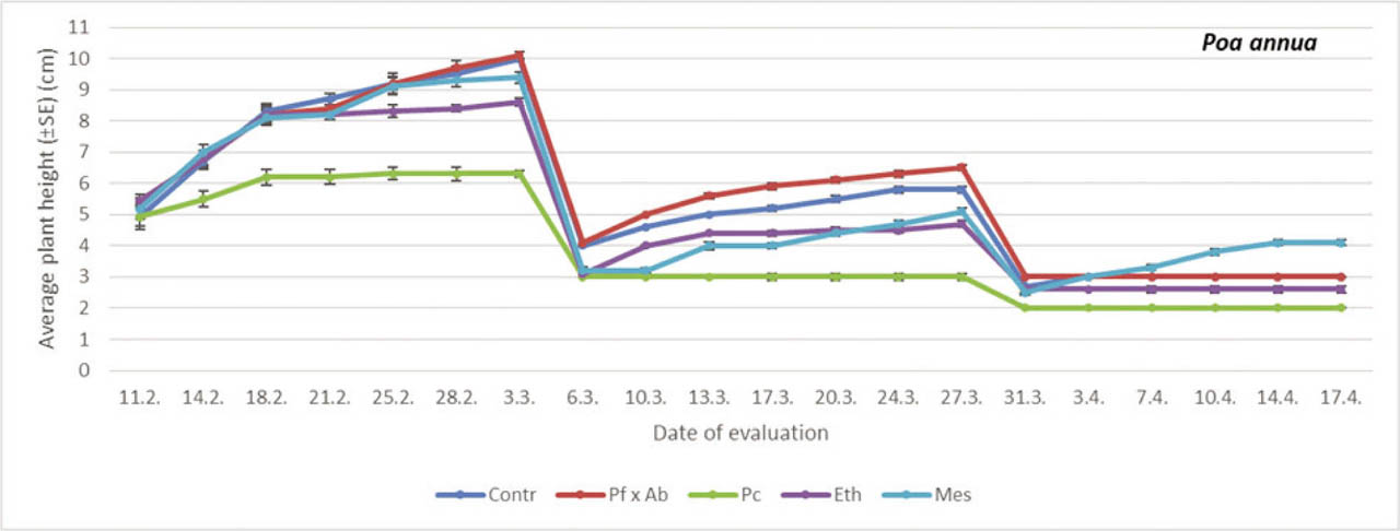
Figure 1
The average plant height on annual bluegrass treated with different PGRs. Within each evaluation date, comparison was done between different treatment (PGRs; Student-Neuman Keuls at p = 0.05). For comparisons within dates, df = 4.24 (11th February, F = 0.62, p = 0.6526; 14th February, F = 7.41, p < 0.05; 18th February, F = 27.76, p < 0.05; 21st February, F = 52.00, p < 0.05; 25th February, F = 110.50, p < 0.05; 28th February, F = 122.37, p < 0.05; 3rd March, F = 84.03, p < 0.05; 6th March, F = 39.57, p < 0.05; 10th March, F = 18.10, p < 0.05; 13th March, F = 16.61, p < 0.05; 17th March, F = 16.10, p < 0.05; 20th March, F = 23.81, p < 0.05; 24th March, F = 4.44, p < 0.05; 27th March, F = 45.97, p < 0.05; 31st March, F = 26.60, p < 0.05; 3rd April, F = 96.00; 7th April, F = 50.40, p < 0.05; 10th April, F = 86.40, p < 0.05; 17th April, F = 65.33, p < 0.05). df, degrees of freedom; Eth, ethephon; F, F-distribution; Mes, mesotrione; Pc, prohexadione calcium; PGRs, plant growth regulators; SE, standard error.
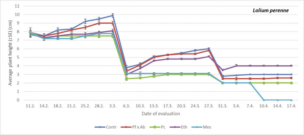
Figure 2
The average plant height on perennial ryegrass treated with different PGRs. Within each evaluation date, a comparison was done between different treatments (PGRs; Student-Neuman Keuls at p = 0.05). For comparisons within dates, df = 4.24 (11th February, F = 0.08, p = 0.9862; 14th February, F = 0.79, p = 0.5435; 18th February, F = 5.96, p < 0.05; 21st February, F = 18.08, p < 0.05; 25th February, F = 26.76, p < 0.05; 28th February, F = 49.53, p < 0.05; 3rd March, F = 35.67, p < 0.05; 6th March, F = 6.30, p < 0.05; 10th March, F = 18.10, p < 0.05; 13th March, F = 26.98, p < 0.05; 17th March, F = 26.37, p < 0.05; 20th March, F = 22.43, p < 0.05; 24th March, F = 18.80, p < 0.05; 27th March, F = 16.65, p < 0.05; 31st March, F = 111.00, p < 0.05; 3rd April, F = 140.00, p < 0.05; 7th April, F = 50.40, p < 0.05; 10th April, F = 116.67, p < 0.05; 17th April, F = 80.76, p < 0.05). df, degrees of freedom; Eth, ethephon; F, F-distribution; Mes, mesotrione; Pc, prohexadione calcium; PGRs, plant growth regulators; SE, standard error.
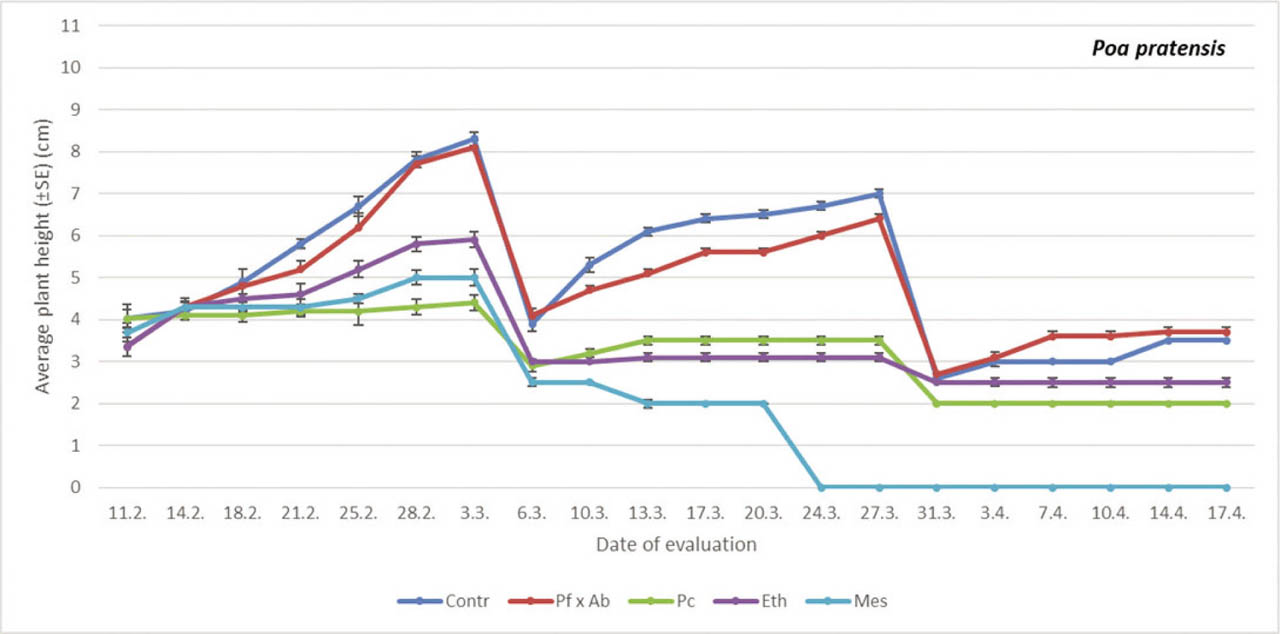
Figure 3
The average plant height in Kentucky treated with different PGRs. Within each evaluation date, a comparison was done between different treatments (PGRs; Student-Neuman Keuls at p = 0.05). For comparisons within dates, df = 4.24 (11th February, F = 2.23, p = 0.1020; 14th February, F = 0.57, p = 0.6864; 18th February, F = 7.47, p < 0.05; 21st February, F = 18.83, p < 0.05; 25th February, F = 27.45, p < 0.05; 28th February, F = 67.49, p < 0.05; 3rd March, F = 109.41, p < 0.05; 6th March, F = 78.67, p < 0.05; 10th March, F = 75.42, p < 0.05; 13th March, F = 102.62, p < 0.05; 17th March, F = 107.32, p < 0.05; 20th March, F = 143.46, p < 0.05; 24th March, F = 73.35, p < 0.05; 27th March, F = 108.69, p < 0.05; 31st March, F = 15.47, p < 0.05; 3rd April, F = 102.67, p < 0.05; 7th April, F = 187.67, p < 0.05; 10th April, F = 187.67, p < 0.05; 17th April, F = 174.89, p < 0.05). df, degrees of freedom; Eth, ethephon; F, F-distribution; Mes, mesotrione; Pc, prohexadione calcium; PGRs, plant growth regulators; SE, standard error.
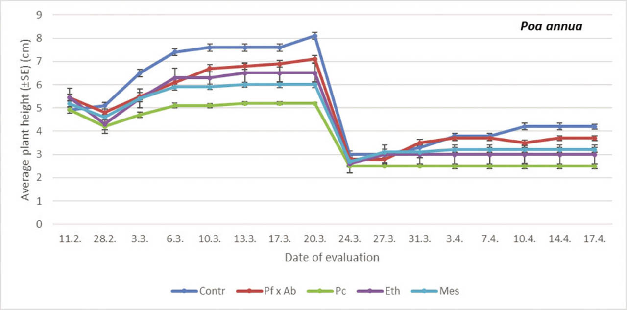
Figure 4
The average plant height on annual bluegrass treated with different PGRs. Within each evaluation date, a comparison was done between different treatments (PGRs; Student-Neuman Keuls at p < 0.05). For comparisons within dates, df = 4.24 (11th February, F = 0.62, p = 0.6526; 28th February, F = 10.38, p < 0.05; 3rd March, F = 12.97, p < 0.05; 6th March, F = 19.11, p < 0.05; 10th March, F = 23.30, p < 0.05; 13th March, F = 24.30, p < 0.05; 17th March, F = 22.24, p < 0.05; 20th March, F = 32.62, p < 0.05; 24th March, F = 13.20, p = 0.0624; 27th March, F = 20.20, p = 0.0523; 31st March, F = 30.30, p < 0.05; 3rd April, F = 26.11, p < 0.05; 7th April, F = 25.13, p < 0.05; 10th April, F = 40.11, p < 0.05; 14th April, F = 52.00, p < 0.05; 17th April, F = 142.37, p < 0.05). df, degrees of freedom; Eth, ethephon; F, F-distribution; Mes, mesotrione; Pc, prohexadione calcium; PGRs, plant growth regulators; SE, standard error.
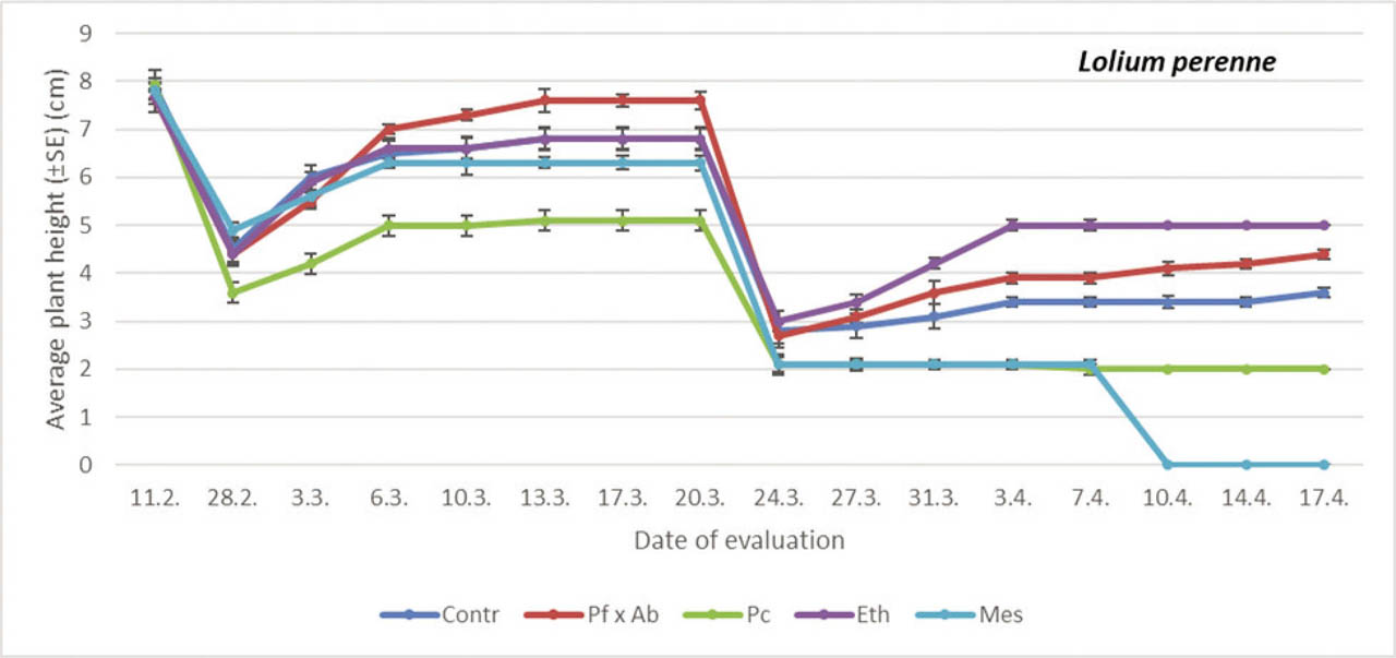
Figure 5
The average plant height on perennial ryegrass treated with different PGRs. Within each evaluation date, a comparison was done between different treatments (PGRs; Student-Neuman Keuls at p < 0.05). For comparisons within dates, df = 4.24 (11th February, F = 5.42, p = 0.0726; 28th February, F = 13.13, p = 0.0595; 3rd March, F = 44.97, p < 0.05; 6th March, F = 39.81, p < 0.05; 10th March, F = 11.30, p < 0.05; 13th March, F = 16.30, p < 0.05; 17th March, F = 33.24, p < 0.05; 20th March, F = 32.62, p < 0.05; 24th March, F = 23.11, p = 0.0724; 27th March, F = 23.26, p = 0.06; 31st March, F = 11.30, p < 0.05; 3rd April, F = 30.11, p < 0.05; 7th April, F = 44.23, p < 0.05; 10th April, F = 30.60, p < 0.05; 14th April, F = 16.00, p < 0.05; 17th April, F = 88.37, p < 0.05). df, degrees of freedom; Eth, ethephon; F, F-distribution; Mes, mesotrione; Pc, prohexadione calcium; PGRs, plant growth regulators; SE, standard error.
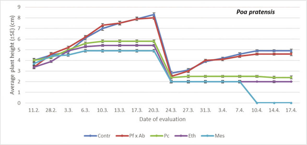
Figure 6
The average plant height on Kentucky bluegrass treated with different PGRs. Within each evaluation date, a comparison was done between different treatments (PGRs; Student-Neuman Keuls at p < 0.05). For comparisons within dates, df = 4.24 (11th February, F = 3.02, p = 0.0626; 28th February, F = 11.26, p = 0.0485; 3rd March, F = 11.97, p < 0.05; 6th March, F = 103.81, p < 0.05; 10th March, F = 151.20, p < 0.05; 13th March, F = 23.30, p < 0.05; 17th March, F = 55.24, p < 0.05; 20th March, F = 32.62, p = 0.0532; 24th March, F = 7.11, p = 0.0814; 27th March, F = 23.26, p = 0.08; 31st March, F = 30.30, p < 0.05; 3rd April, F = 25.11, p < 0.05; 7th April, F = 38.23, p < 0.05; 10th April, F = 30.60, p < 0.05; 14th April, F = 32.00, p < 0.05; 17th April, F = 30.37, p < 0.05). df, degrees of freedom; Eth, ethephon; F, F-distribution; Mes, mesotrione; Pc, prohexadione calcium; PGRs, plant growth regulators; SE, standard error.
Table 4
Repeated measures ANOVA parameters for the main effects and associated interaction for average tiller number.
| Source between variables | df | F | p |
|---|---|---|---|
| All between | 28 | 88.1 | <0.05 |
| Intercept | 1 | 77.1 | <0.05 |
| Treatment | 4 | 109.8 | <0.05 |
| Turfgrass species | 2 | 145.2 | <0.05 |
| Experiment type | 1 | 11.6 | <0.05 |
| Treatment × turfgrass species | 8 | 14.7 | <0.05 |
| Turfgrass species × experiment type | 4 | 4.7 | <0.05 |
| Treatment × turfgrass species × experiment type | 8 | 12.3 | <0.05 |
| Source within Experiment 1 | |||
| Within interactions | 126 | 87.3 | <0.05 |
| Date of evaluation | 18 | 40.9 | <0.05 |
| Date of evaluation × treatment | 72 | 4.9 | <0.05 |
| Date of evaluation × turfgrass species | 36 | 3.4 | <0.05 |
| Source within Experiment 2 | |||
| Within interactions | 98 | 65.1 | <0.05 |
| Date of evaluation | 14 | 55.3 | <0.05 |
| Date of evaluation × treatment | 56 | 44.4 | <0.05 |
| Date of evaluation × turfgrass species | 28 | 25.1 | <0.05 |
[i] df – degrees of freedom; F – F-distribution is a continuous probability distribution that arises frequently as the null distribution of test statistics; p – p-value as probability of obtaining test results at least as extreme as the results observed under the assumption that the null hypothesis is correct.
[ii] ANOVA, analysis of variance.
Table 5
Repeated measures ANOVA parameters for the main effects and associated interactions for average tiller number per plant within turfgrass species in Experiments 1 and 2 (error df = 474).
| Experiment type | Source | df | F | p |
|---|---|---|---|---|
| 1 | Sources within annual bluegrass | |||
| Date of evaluation | 18 | 11.7 | <0.05 | |
| Treatment | 4 | 43.3 | <0.05 | |
| Date of evaluation × treatment | 72 | 2.9 | <0.05 | |
| Source within perennial ryegrass | ||||
| Date of evaluation | 18 | 19.9 | <0.05 | |
| Treatment | 4 | 50.7 | <0.05 | |
| Date of evaluation × treatment | 72 | 2.7 | <0.05 | |
| Source within Kentucky bluegrass | ||||
| Date of evaluation | 18 | 13.3 | <0.05 | |
| Treatment | 4 | 44.4 | <0.05 | |
| Date of evaluation × treatment | 72 | 13.3 | <0.05 | |
| 2 | Sources within annual bluegrass | |||
| Date of evaluation | 14 | 4.4 | <0.05 | |
| Treatment | 4 | 24.8 | <0.05 | |
| Date of evaluation × treatment | 56 | 3.8 | <0.05 | |
| Source within perennial ryegrass | ||||
| Date of evaluation | 14 | 4.7 | <0.05 | |
| Treatment | 4 | 25.6 | <0.05 | |
| Date of evaluation × treatment | 56 | 2.7 | <0.05 | |
| Source within Kentucky bluegrass | ||||
| Date of evaluation | 18 | 3.0 | <0.05 | |
| Treatment | 4 | 22 | <0.05 | |
| Date of evaluation × treatment | 72 | 13.33 | <0.05 |
[i] df – degrees of freedom; F – F-distribution is a continuous probability distribution that arises frequently as the null distribution of test statistics; p – p-value as probability of obtaining test results at least as extreme as the results observed under the assumption that the null hypothesis is correct.
[ii] ANOVA, analysis of variance.
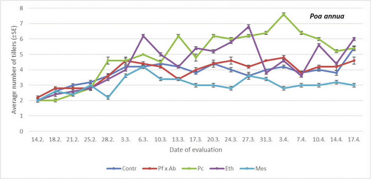
Figure 7
The average number of tillers on annual bluegrass treated with different PGRs. Within each evaluation date, a comparison was done between different treatments (PGRs; Student-Neuman Keuls at p < 0.05). For comparisons within dates, df = 4.24 (14th February, F = 3.02, p = 0.0626; 18th February, F = 0.57, p = 0.0485; 21st February, F = 0.50, p = 0.7360; 25th February, F = 3.30, p = 0.0623; 28th February, F = 30.40, p < 0.05; 3rd March, F = 0.88, p < 0.05; 6th March, F = 4.56, p < 0.05; 10th March, F = 4.23, p < 0.05; 13th March, F = 6.87, p < 0.05; 17th March, F = 5.63, p < 0.05; 20th March, F = 5.63, p < 0.05; 24th March, F = 6.19, p < 0.05; 27th March, F = 23.62 p < 0.05; 31st March, F = 2.71, p < 0.0591; 3rd April, F = 20.11, p < 0.05; 7th April, F = 7.25, p < 0.05; 10th April, F = 81.15, p < 0.05; 17th April, F = 30.11, p < 0.05). df, degrees of freedom; Eth, ethephon; F, F-distribution; Mes, mesotrione; Pc, prohexadione calcium; PGRs, plant growth regulators; SE, standard error.
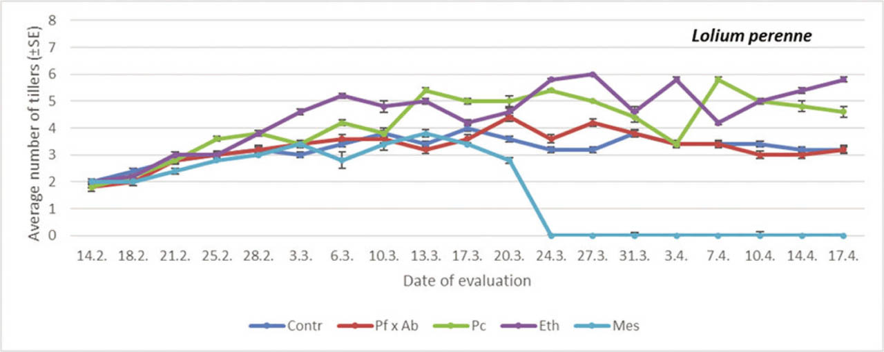
Figure 8
The average number of tillers on perennial ryegrass treated with different PGRs. Within each evaluation date, a comparison was done between different treatments (PGRs; Student-Neuman Keuls at p < 0.05). For comparions within date, df = 4.24 (14th February, F = 0.0723, p < 0.05; 18th February, F = 2.09, p = 0.1200; 21st February, F = 1.55, p = 0.2274; 25th February, F = 12.12, p = 0.2236; 28th February, F = 13.07, P < 0.05; 3rd March, F = 1.10, p < 0.05; 6th March, F = 7.50, p < 0.05; 10th March, F = 10.10, p = 0.0564; 13th March, F = 19.29, p < 0.05; 17th March, F = 3.21, p = 0.0345; 20th March, F = 6.31, p < 0.05; 24th March, F = 4.75, p < 0.05; 27th March, F = 30.30, p < 0.05; 31st March, F = 21.70, p < 0.05; 3rd April, F = 15.08, p < 0.05; 7th April, F = 25.40, p < 0.05; 10th April, F = 61.13, p < 0.05; 14th April, F = 61.13, p < 0.05; 17th April, F = 33.15; p < 0.05). df, degrees of freedom; Eth, ethephon; F, F-distribution; Mes, mesotrione; Pc, prohexadione calcium; PGRs, plant growth regulators; SE, standard error.
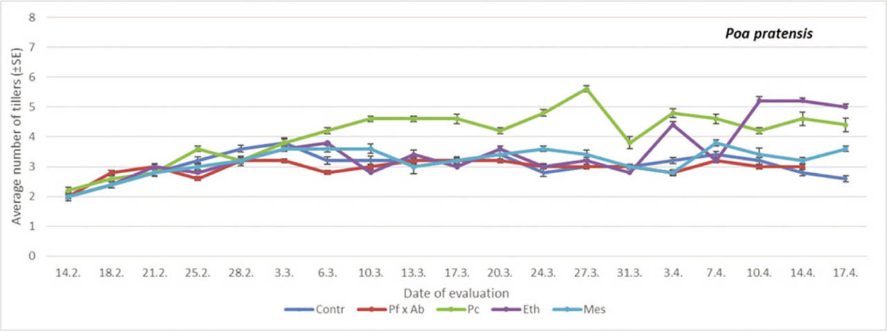
Figure 9
The average number of tillers on Kentucky bluegrass treated with different PGRs. Within each evaluation date, a comparison was done between different treatments (PGRs; Student-Neuman Keuls at p < 0.05). For comparisons within date, df = 4.24 (14th February, F = 3.09, p < 0.05; 18th February, F = 2.09, p = 0.7200; 21st February, F = 1.55, p = 0.2274; 25th February, F = 30.12, p = 0.7236; 28th February, F = 20.07, p < 0.05; 3rd March, F = 1.10, p < 0.05; 6th March, F = 7.50, p < 0.05; 10th March, F = 10.10, p = 0.0564; 13th March, F = 19.29, p < 0.05; 17th March, F = 3.21, p = 0.0345; 20th March, F = 6.31, p < 0.05; 24th March, F = 4.75, p < 0.05; 27th March, F = 30.30, p < 0.05; 31st March, F = 21.70, p < 0.05; 3rd April, F = 15.08, p < 0.05; 7th April, F = 75.40, p = 0.0935; 10th April, F = 61.13, p < 0.05; 14th April, F = 77.13, p < 0.05; 17th April, F = 37.15; p < 0.05). df, degrees of freedom; Eth, ethephon; F, F-distribution; Mes, mesotrione; Pc, prohexadione calcium; PGRs, plant growth regulators; SE, standard error.
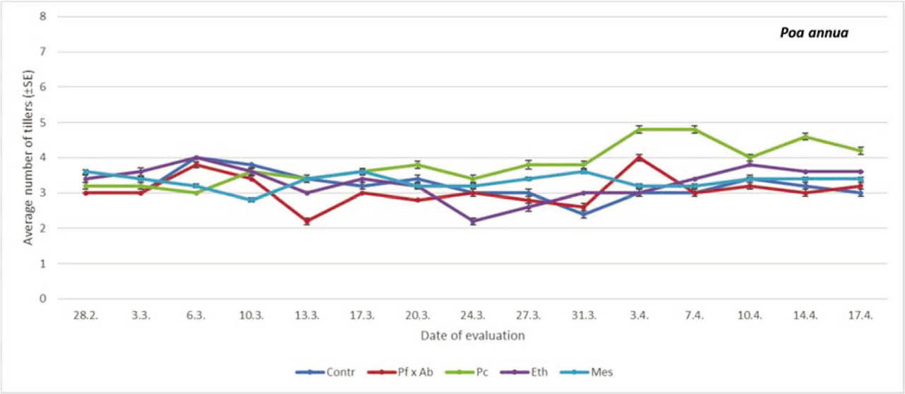
Figure 10
The average number of tillers on annual bluegrass treated with different PGRs. Within each evaluation date, comparison was done between different treatment (PGRs; Student-Neuman Keuls at p < 0.05). For comparisons within dates, df = 4.24 (28th February, F = 9.06, p = 0.0936; 3rd March, F = 7.38, p < 0.05; 6th March, F = 4.56, p < 0.05; 10th March, F = 4.23, p < 0.05; 13th March, F = 13.87, p < 0.05; 17th March, F = 77.33, p < 0.05; 20th March, F = 130.63, p < 0.05; 24th March, F = 31.19, p < 0.05; 27th March, F = 66.62 p < 0.05; 31st March, F = 77.71, p < 0.05; 3rd April, F = 220.11, p < 0.05; 7th April, F = 34.25, p < 0.05; 10th April, F = 111.15, p < 0.05; 17th April, F = 230.11, p < 0.05). df, degrees of freedom; Eth, ethephon; F, F-distribution; Mes, mesotrione; Pc, prohexadione calcium; PGRs, plant growth regulators; SE, standard error.
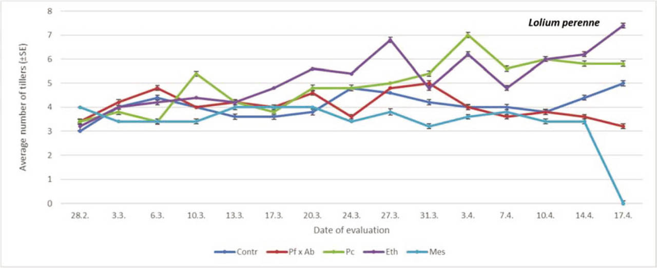
Figure 11
The average number of tiller on perennial ryegrass treated with different PGRs. Within each evaluation date, comparison was done between different treatments (PGRs; Student-Neuman Keuls at p < 0.05). For comparions within date, df = 4.24 (28th February, F = 17.06, p = 0.0936; 3rd March, F = 7.38, p = 0.2005; 6th March, F = 4.56, p < 0.05; 10th March, F = 4.23, p < 0.05; 13th March, F = 22.87, p < 0.05; 17th March, F = 77.33, p < 0.05; 20th March, F = 130.63, p < 0.05; 24th March, F = 70.16, p < 0.05; 27th March, F = 30.11, p < 0.05; 31st March, F = 13.71, p < 0.05; 3rd April, F = 70.11, p < 0.05; 7th April, F = 130.35, p < 0.05; 10th April, F = 17.15, p < 0.05; 17th April, F = 90.11, p < 0.05). df, degrees of freedom; Eth, ethephon; F, F-distribution; Mes, mesotrione; Pc, prohexadione calcium; PGRs, plant growth regulators; SE, standard error.
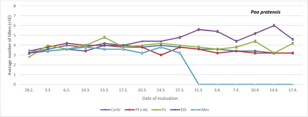
Figure 12
The average number of tillers per plant on Kentucky bluegrass treated with different PGRs. Within each evaluation date, comparison was done between different treatments (PGRs; Student-Neuman Keuls at p < 0.05). For comparions within date, df = 4.24 (28th February, F = 7.03, p = 0.0636; 3rd March, F = 9.33, p = 0.4005; 6th March, F = 9.53, p = 0.5246; 10th March, F = 9.23, p < 0.05; 13th March, F = 22.87, p = 0.0563; 17 th March, F = 7.23, p = 0.0625; 20th March, F = 30.11, p < 0.05; 24th March, F = 70.16, p < 0.05; 27th March, F = 11.11, p < 0.05; 31st March, F = 143.61, p < 0.05; 3rd April, F = 270.11, p < 0.05; 7th April, F = 136.31, p < 0.05; 10th April, F = 141.15, p < 0.05; 17th April, F = 90.11, p < 0.05). df, degrees of freedom; Eth, ethephon; F, F-distribution; Mes, mesotrione; Pc, prohexadione calcium; PGRs, plant growth regulators; SE, standard error.
Table 6
Plant height ratio of three turfgrass species across five treatments and three growth periods – Experiment 1.
| Turfgrass species | Treatment | Period | ||
|---|---|---|---|---|
| 3rd Mar/11th Feb | 27th Mar/6th Mar | 17th Apr/31st Mar | ||
| Annual bluegrass | Contr | 2.03 | 1.45 | 1.10 |
| Pf × Ab | 1.86 | 1.58 | 1.00 | |
| Pc | 1.28 | 1.00 | 1.00 | |
| Eth | 1.58 | 1.52 | 1.00 | |
| Mes | 1.81 | 1.52 | 1.00 | |
| Perennial ryegrass | Contr | 1.25 | 1.58 | 1.07 |
| Pf × Ab | 1.17 | 1.71 | 1.04 | |
| Pc | 0.94 | 1.20 | 1.00 | |
| Eth | 1.05 | 1.17 | 1.14 | |
| Mes | 1.00 | 1.00 | – | |
| Kentucky bluegrass | Contr | 2.06 | 1.80 | 1.35 |
| Pf × Ab | 2.41 | 1.57 | 1.37 | |
| Pc | 1.09 | 1.21 | 1.00 | |
| Eth | 1.75 | 1.03 | 1.00 | |
| Mes | 1.35 | – | – | |
[i] (−) because of the high efficacy of the product, we could not calculate the ratio; Feb – February; Mar – March; Apr – April.
[ii] Eth, ethephon; Mes, mesotrione; Pc, prohexadione calcium.
Table 8
Plant height ratio of three turfgrass species across five treatments and two growth periods – Experiment 2.
| Turfgrass species | Treatment | Period | |
|---|---|---|---|
| 20th Mar/28th Feb | 17th Apr/23rd Mar | ||
| Annual bluegrass | Contr | 1.62 | 1.40 |
| Pc × Ab | 1.48 | 1.32 | |
| Pc | 1.24 | 1.00 | |
| Eth | 1.52 | 1.15 | |
| Mes | 1.30 | 1.18 | |
| Perennial ryegrass | Contr | 1.52 | 1.28 |
| Pc × Ab | 1.73 | 1.63 | |
| Pc | 1.42 | 0.95 | |
| Eth | 1.54 | 1.68 | |
| Mes | 1.28 | – | |
| Kentucky bluegrass | Contr | 1.84 | 1.75 |
| Pc × Ab | 1.74 | 1.84 | |
| Pc | 1.35 | 1.02 | |
| Eth | 1.38 | 1.00 | |
| Mes | 1.11 | – | |
[i] (−) because of the high efficacy of the product, we could not calculate the ratio; Feb – February; Mar – March; Apr – April.
[ii] Eth, ethephon; Mes, mesotrione; Pc, prohexadione calcium.
Table 9
Tillers ratio of three turfgrass species across five treatments and two growth periods – Experiment 2.
| Turfgrass species | Treatment | Period | |
|---|---|---|---|
| 20th Mar/28th Feb | 17th Apr/23rd Mar | ||
| Annual bluegrass | Contr | 1.13 | 1.00 |
| Pc × Ab | 0.93 | 1.06 | |
| Pc | 1.19 | 1.23 | |
| Eth | 0.94 | 1.63 | |
| Mes | 0.89 | 1.06 | |
| Perennial ryegrass | Contr | 1.26 | 1.04 |
| Pc × Ab | 1.35 | 0.89 | |
| Pc | 1.42 | 1.21 | |
| Eth | 1.75 | 1.37 | |
| Mes | 1.00 | – | |
| Kentucky bluegrass | Contr | 1.19 | 0.80 |
| Pc × Ab | 1.12 | 1.06 | |
| Pc | 1.43 | 1.00 | |
| Eth | 1.37 | 1.04 | |
| Mes | 0.94 | – | |
[i] (−) because of the high efficacy of the product, we could not calculate the ratio; Feb – February; Mar – March; Apr – April.
[ii] Eth, ethephon; Mes, mesotrione; Pc, prohexadione calcium.