
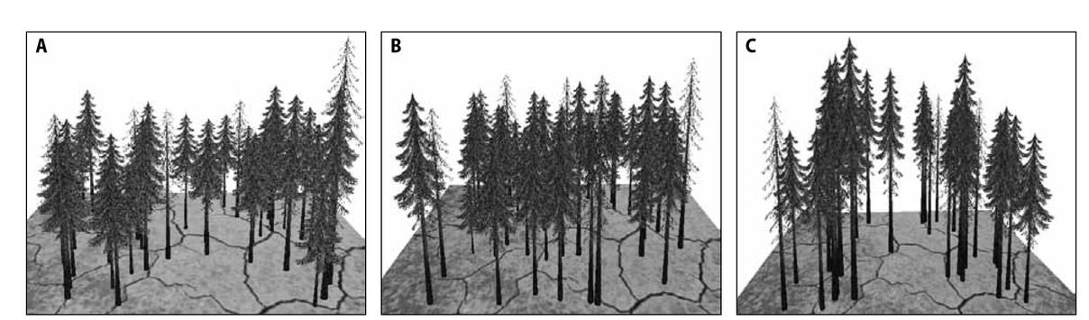
Figure 1
Three-dimensional visualisation of Norway spruce stands occurring on the sample plots at the beginning of simulation (A, B and C –plot nos. 1, 2 and 3, respectively)
Table 1
Basic characteristics of spruce trees occurring on study plots
| Plot | DBH1.3 [cm] | H [m] | Mean age [years] | n | ||||
|---|---|---|---|---|---|---|---|---|
| mean | min. | max. | mean | min. | max. | |||
| 1 | 20.3 | 8.0 | 32.0 | 19.2 | 5.5 | 24.5 | 43 | 35 |
| 2 | 22.4 | 10.5 | 33.5 | 19.4 | 6.5 | 24.0 | 46 | 34 |
| 3 | 25.9 | 13.5 | 36.5 | 21.8 | 7.0 | 25.0 | 51 | 25 |
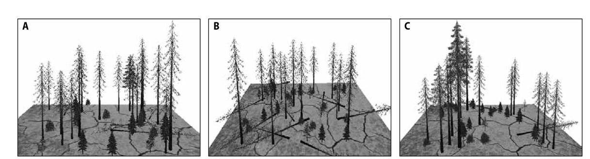
Figure 2
Three-dimensional views of the sample plotsat the 10th year of simulation time(A, B and C – plot nos. 1, 2 and 3, respectively)
Table 2
Stand biomass by tree species for different scenarios in the 50th year of simulation
| Species | Scenario | ||||
|---|---|---|---|---|---|
| control | 1 | 2 | 3 | 4 | |
| Plot 1 | |||||
| Fagus sylvatica | 101.3 ± 5.6 | 60.9 ± 3.7 | 98.5 ± 4.1 | 109.6 ± 6.1 | 188.8 ± 6.9 |
| Abies alba | 23.8 ± 2.7 | 10.4 ± 1.1 | 25.8 ± 2.9 | 26.8 ± 3.1 | 51.3 ± 0.9 |
| Picea abies | 0.3 ± 0.1 | 0.2 ± 0.1 | 0.2 ± 0.1 | 0.2 ± 0.1 | 0.3 ± 0.1 |
| Plot 2 | |||||
| Fagus sylvatica | 103.9 ± 3.4 | 61.6 ± 1.1 | 90,1 ± 4.1 | 105.2 ± 1.8 | 199.9 ± 6.7 |
| Abies alba | 26.4 ± 0.4 | 11.2 ± 0.2 | 29.5 ± 0.1 | 26.9 ± 0.4 | 50.4 ± 1.6 |
| Picea abies | 0.3 ± 0.1 | 0.2 ± 0.1 | 0.2 ± 0.1 | 0.2 ± 0.1 | 0.3 ± 0.1 |
| Plot 3 | |||||
| Fagus sylvatica | 108.0 ± 4.6 | 62.5 ± 3.4 | 99.6 ± 6.1 | 110.6 ± 6.1 | 196.4 ± 6.3 |
| Abies alba | 25.8 ± 2.7 | 12.4 ± 0.9 | 27.6 ± 3.2 | 26.8 ± 3.1 | 52.7 ± 1.2 |
| Picea abies | 0.2 ± 0.1 | 0.2 ± 0.1 | 0.2 ± 0.1 | 0.2 ± 0.1 | 0.2 ± 0.1 |
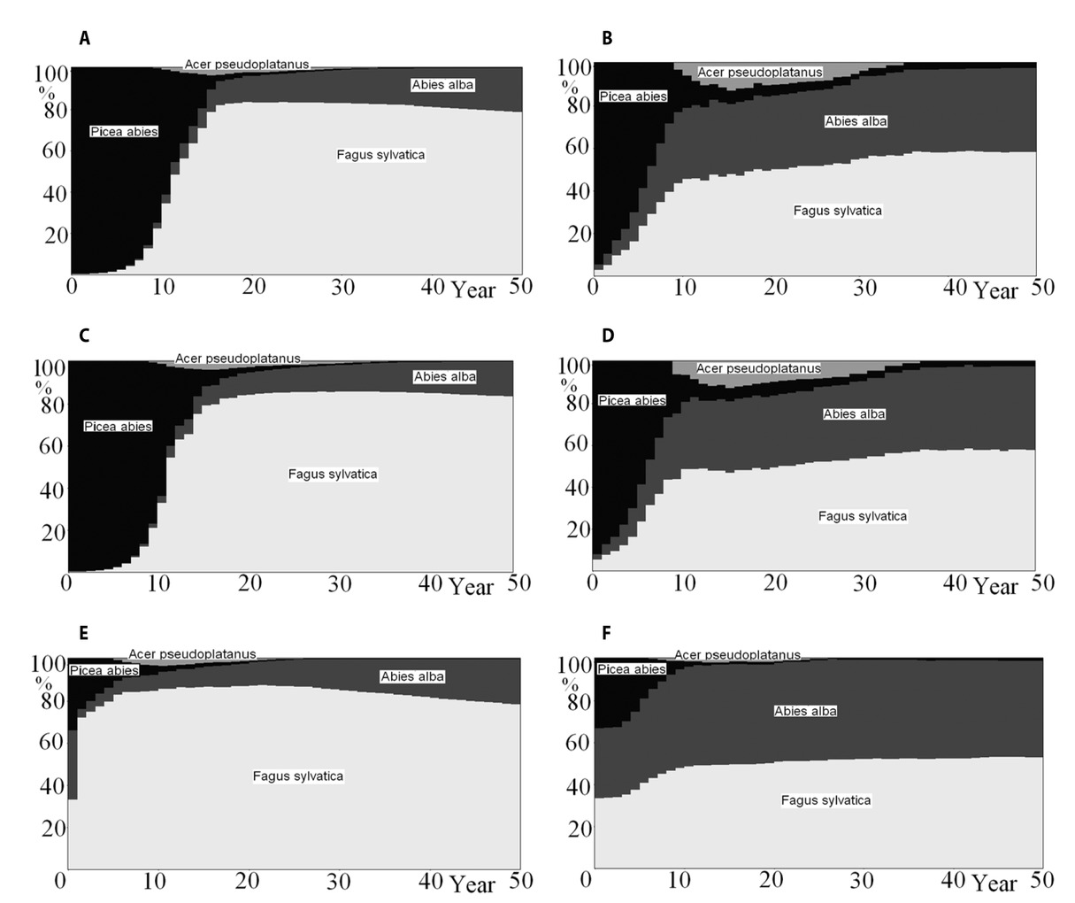
Figure 3
Temporal changes in the share of biomass (left panel) and the number of trees (right panel) in control (A, B) and in the first (C, D) and fourth (E, F) scenarios for plot 2
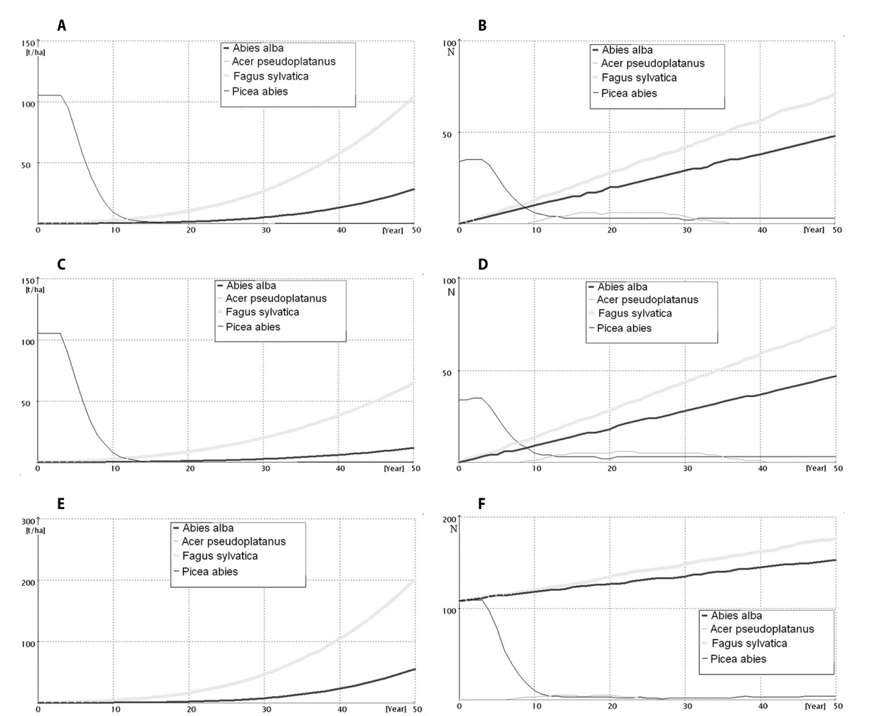
Figure 4
Prediction of biomass (left panel) and number of trees (right panel) in control (A, B), in the first (C, D) and fourth (E, F) scenarios for plot 2
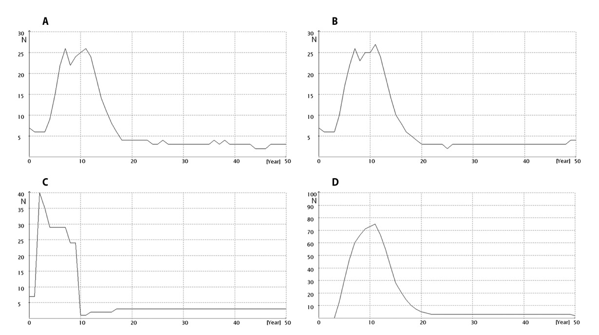
Figure 5
Number of dead trees in the simulations conducted for plot 2 (A – control, B – first scenario, C – third scenario, D – fourth scenario)
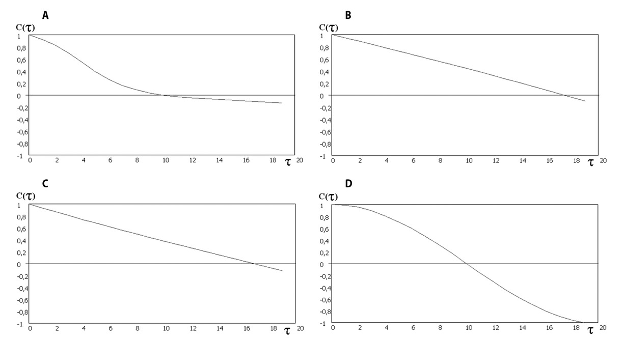
Figure 6
Auto-correlation of biomass in control conditions for spruce (A), beech (B), fir (C) and sycamore (D) (τ – Kendall coefficient)
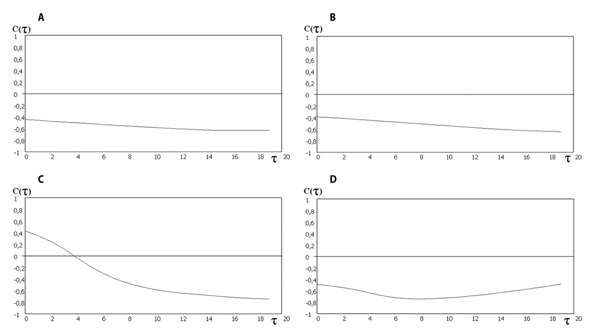
Figure 7
Cross-correlations in the control scenario: between spruce and beech biomass (A), between spruce and fir biomass (B), between spruce and total stand biomass (C), between spruce tree number and total stand density (D) (τ – Kendall coefficient)