
Fig. 1
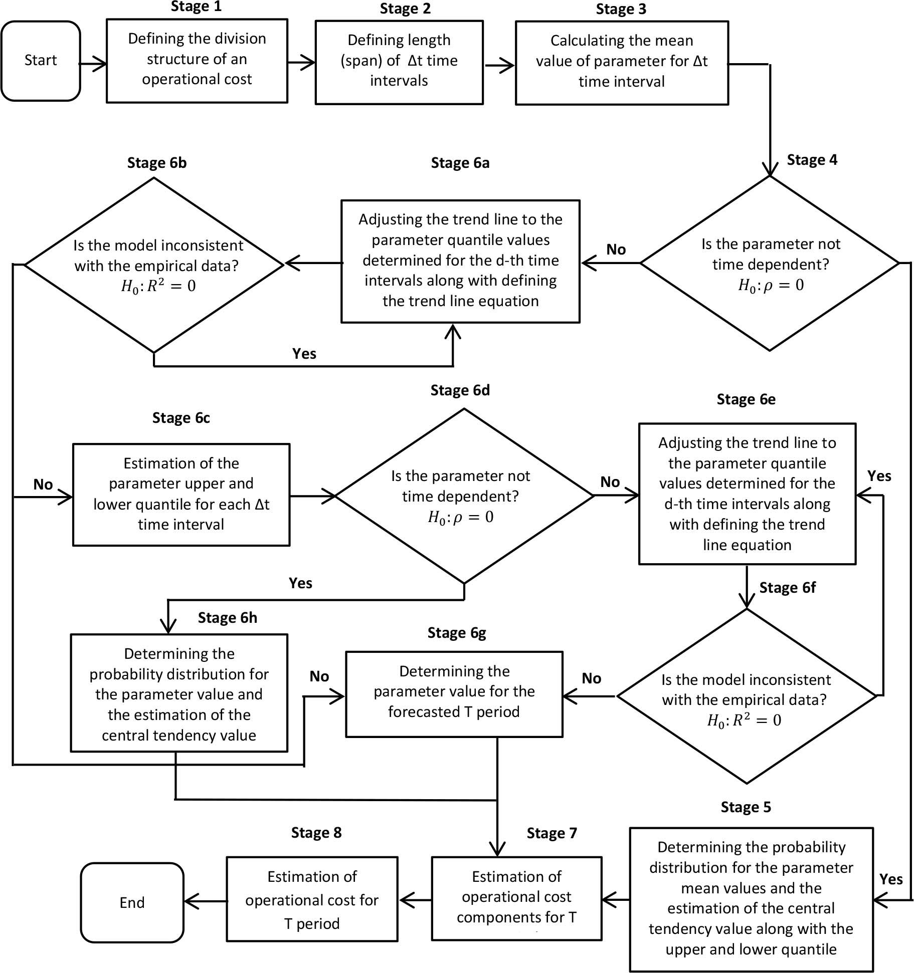
Fig. 2
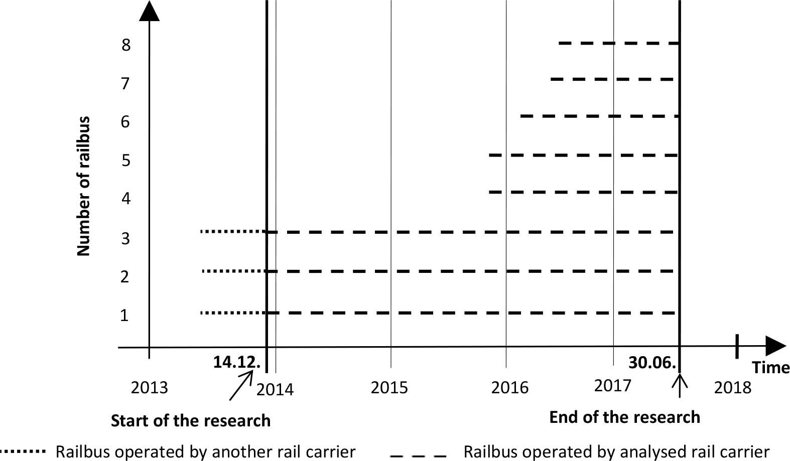
Fig. 3
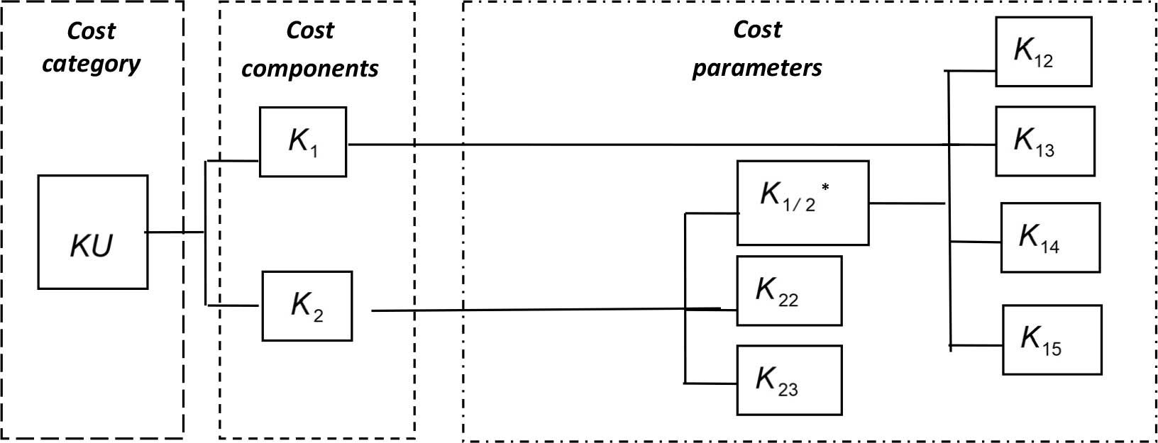
Fig. 4
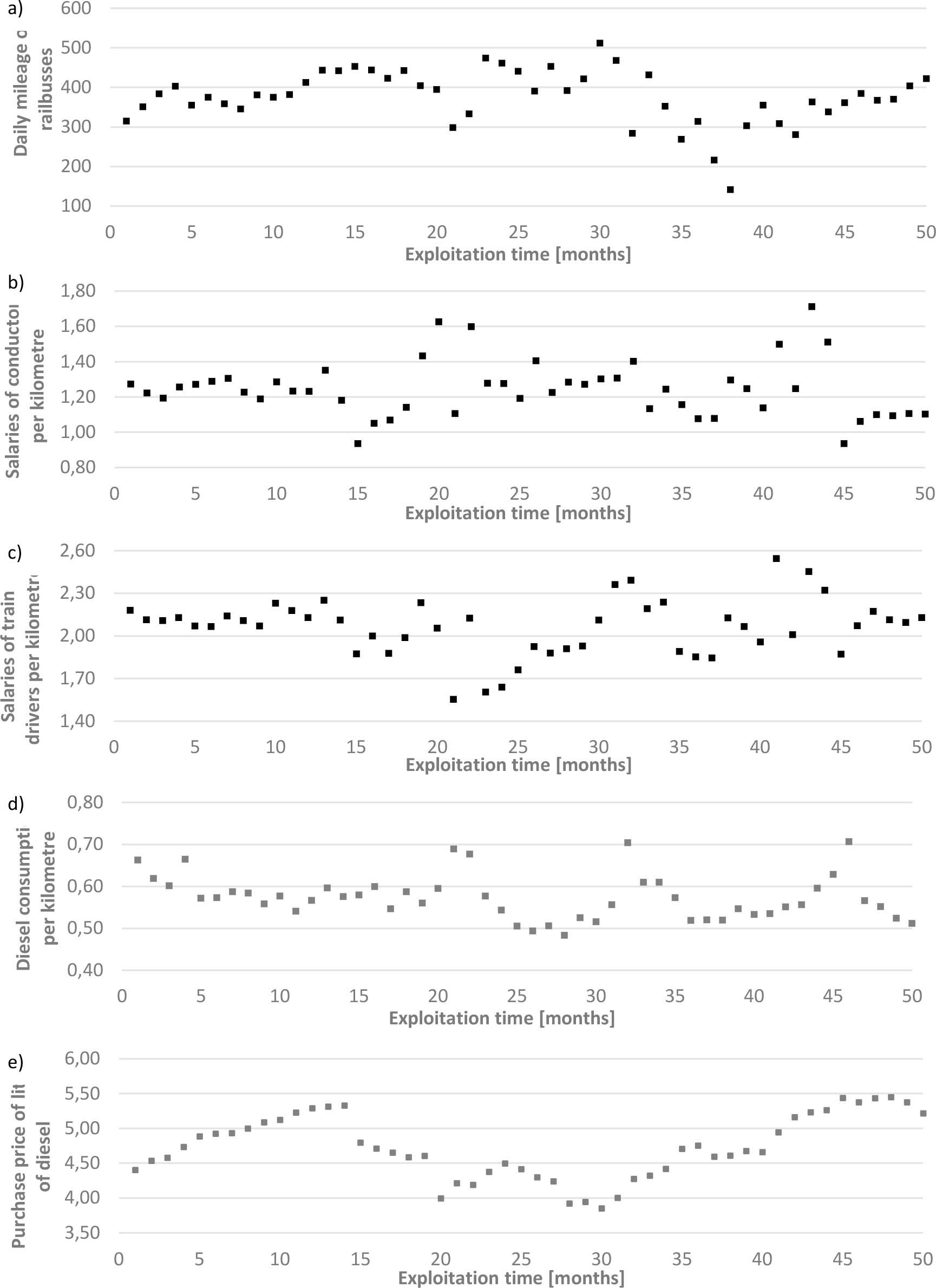
Fig. 5
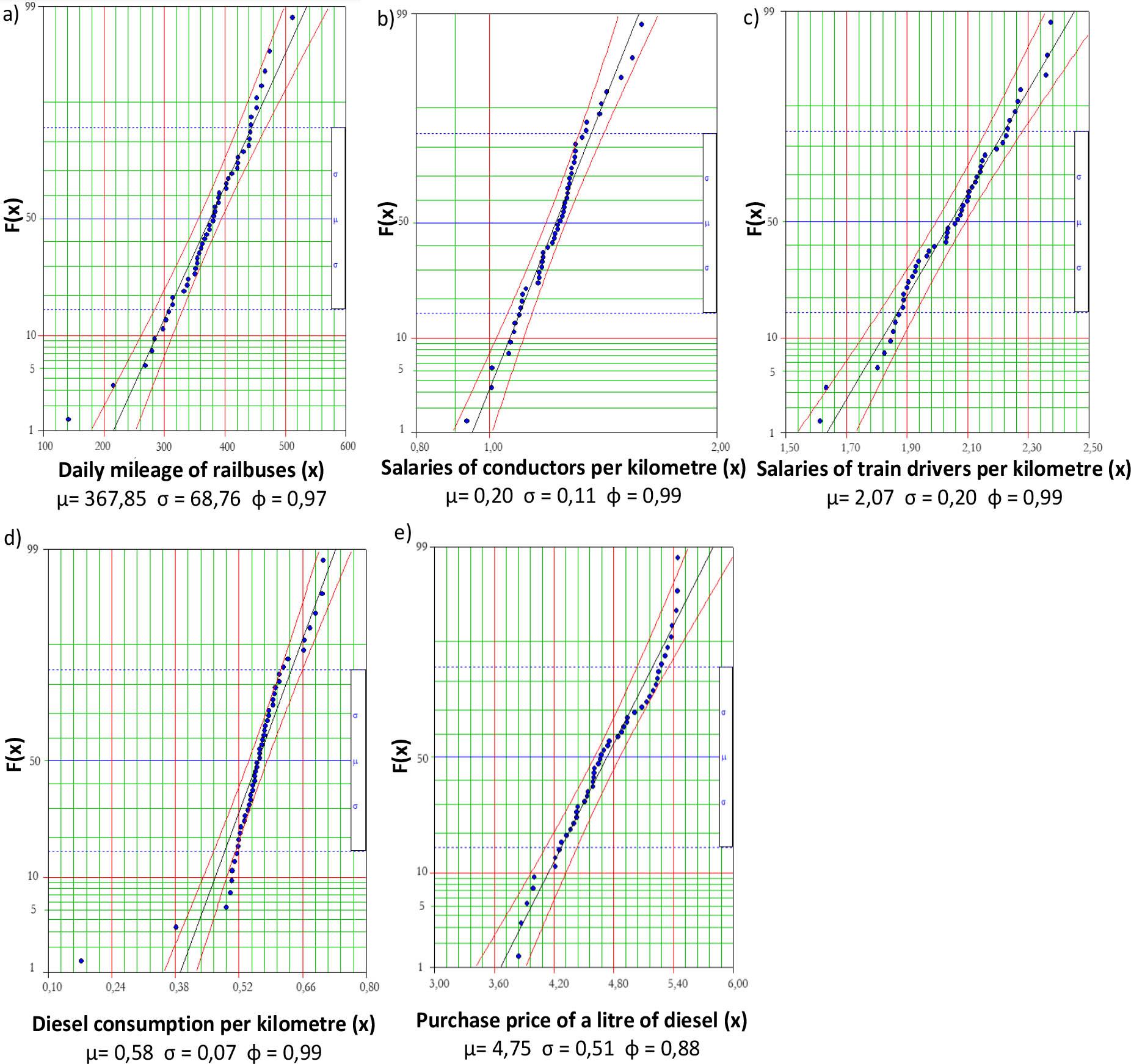
Fig. 6
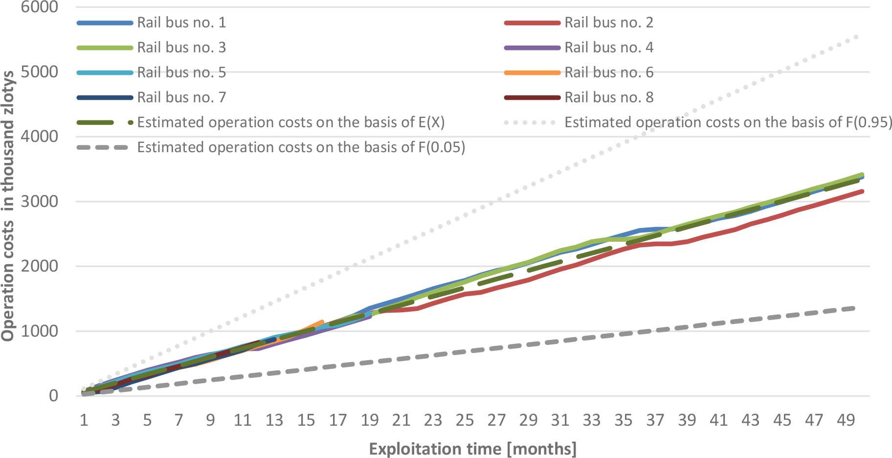
Relative errors in measuring operational costs of railbuses
| R | L | KUt | γt | M | |
|---|---|---|---|---|---|
| 1 | 50 | 3379357 | 3340998 | −1.1% | 2.9% |
| 2 | 50 | 3156515 | 3340998 | 5.5% | |
| 3 | 50 | 3416362 | 3340998 | −2.3% | |
| 4 | 19 | 1226472 | 1269579 | 3.4% | |
| 5 | 19 | 1276996 | 1269579 | −0.58% | |
| 6 | 16 | 1140901 | 1069119 | −6.7% | |
| 7 | 13 | 873708 | 868659 | −0.58% | |
| 8 | 12 | 825694 | 801839 | −3.0% |
Parameters of the operational cost components for time intervals presented as the months of vehicle exploitation
| P | ||||||
|---|---|---|---|---|---|---|
| K1/2 | K12 | K14 | K22 | K23 | ||
| S | Correlation coefficient (r) | −0.22 | −0.07 | 0.06 | 0.18 | −0.25 |
| For ∝= 0,05 | t = −1.59 | t = −0.51 | t = 0.45 | t =1.27 | t = −1.78 | |
| Accepted hypothesis | H0: ρ = 0 | H0: ρ = 0 | H0: ρ = 0 | H0: ρ = 0 | H0: ρ = 0 | |
| S | Type of probability distribution | Normal | Log-normal | Normal | Normal | Normal |
| Distribution matching (φ) | 0.97 | 0.99 | 0.99 | 0.99 | 0.88 | |
| E(X) | 367.85 | 1.23 | 2.07 | 4.75 | 0.58 | |
| F(x0,95) | 480.95 | 1.46 | 2.41 | 5.60 | 0.69 | |
| F(x0,05) | 254.76 | 0.02 | 1.72 | 3.91 | 0.47 | |