
Table 1:
Variables used in the study and their definition.
| Variable | Characteristic | Definition |
|---|---|---|
| LNTOUR | The logarithm of international tourism receipts | International tourism receipts (currency US$) |
| LNGDPG | The logarithm of gross domestic product (GDP) growth | GDP growth (annual %) |
| LNREER | The logarithm of the real effective exchange rate | Real effective exchange rate index (2010 = 100) |
1 Source: The variables are related to Algeria, and all data are from the World Development Indicators’ Data Bank by the World Bank https://databank.worldbank.org/reports.aspx?source=world-development-indicators, except for LNTOUR (1990–1994, 2018, 2019) and LNGDPG (2019), which we obtained from the Algerian National Bureau of Statistics (www.ons.dz).
Table 2:
Descriptive statistics of the variables in the study.
| LNGDPG | LNTOUR | LNREER | |
|---|---|---|---|
| M | 4.631941 | 4.731771 | 18.64382 |
| Median | 4.63574 | 4.637684 | 18.98015 |
| Maximum | 4.674714 | 5.396235 | 19.98303 |
| Minimum | 4.583947 | 4.535622 | 16.86003 |
| SD | 0.020151 | 0.188400 | 1.056439 |
| Probability | 0.693189 | 0.000001 | 0.225635 |
| Sum | 138.9582 | 141.9531 | 559.3146 |
| Observations | 30 | 30 | 30 |
Table 3:
Correlation of the variables in the study.
| LNGDPG | LNREER | LNTOUR | |
|---|---|---|---|
| LNGDPG | 1 | ||
| LNREER | −0.40829842 | 1 | |
| LNTOUR | 0.43076231 | −0.80311554 | 1 |
Table 4:
Unit root test results.
Table 5:
Computed F statistic for cointegration tests—ARDL bounds tests.
| ] I(0)–I(1)] | Conclusion | |||
|---|---|---|---|---|
| Lower–upper bound (10%) | 2.63–3.35 | Cointegration | ||
| Lower–upper bound (5%) | 3.10–3.87 | Cointegration | ||
| Lower–upper bound (1%) | 4.13–5.00 | Cointegration | ||
| DV: LNTOUR | F statistics | 4.44* | ||
| DV: LNGDPG | F statistics | 2.25 | ||
| DV: LNREER | F statistics | 4.63 | ||
| K | 2 | |||
Table 6:
Long-term coefficients estimation with ARDL bounds test model.
| Model | Variable | Coefficient | p-value | |
|---|---|---|---|---|
| ARDL | Dependent variable | LNTOUR | ||
| Independent variable | LNREER | −3.42 | 0.1545 | |
| LNGDPG | 37.53 | 0.1193 | ||
| C | 138.67 | 0.2423 | ||
| ARDL | Dependent variable | LNGDPG | ||
| Independent variable | LNREER | 0.085 | 0.5482 | |
| LNTOUR | 0.0169 | 0.3703 | ||
| C | 3.9 | 0.0008 | ||
| ARDL | Dependent variable | LNREER | ||
| Independent variable | LNTOUR | −0.05 | 0.4 | |
| LNGDPG | −0.52 | 0.82 | ||
| C | 8.03 | 0.45 |
Table 7:
Error correction representation of ARDL bounds test model.
| Model | Variable | Coefficient | p-value | |
|---|---|---|---|---|
| ARDL | Dependent variable | LNTOUR | ||
| ΔLNREER | 0.056 | 0.94 | ||
| Independent variable | ΔLNREERt-1 | 1.07** | 0.0305 | |
| ECTt-1 | −0.263*** | 0.002 | ||
| ARDL | Dependent variable | LNGDPG | ||
| ΔLNTOUR | 0.024*** | 0.0032 | ||
| ΔLNTOURt-1 | −0.017** | 0.0386 | ||
| Independent variable | ΔLNREER | −0.12*** | 0.0044 | |
| ΔLNREERt-1 | −0.062*** | 0.0043 | ||
| ECTt-1 | −0.41*** | 0.0043 | ||
| ARDL | Dependent variable | LNREER | ||
| ΔLNREERt-1 | 0.053 | 0.63 | ||
| Independent variable | ΔLNREERt-2 | −0.41*** | 0.000 | |
| ECTt-1 | −0.25*** | 0.0002 |
Table 8:
VECM Granger causality analysis.
| IV/DV | Long-term | Short-term | ||
|---|---|---|---|---|
| ΔLGDPG | LNREER | ΔLNTOUR | ECTt-1 | |
| ΔLGDPG | – | −0.25 (0.66) | 5.9* (0.07) | −1.68*** (0.00) |
| LNREER | −0.12*** (00092) | – | 0.35 (0.43) | −0.17*** (0.0002) |
| ΔLNTOUR | 0.01 (0.14) | 0.01 (0.71) | – | −0.98*** (0.00) |
| C | −0.166 (0.12) | 0.79 (0.02) | −1.58 (0.45) | – |
| Observations | 27 | 27 | 27 | – |
| R2 | 0.71 | 0.92 | 0.16 | – |
| DW | 1.78 | 1.83 | 1.96 | – |
| Fisher | 6.81*** (00003) | 48.70*** (0.00) | 1.57(0.22) | – |
Table 9:
Diagnostic tests.
| Diagnostic test | LM test | ARCH test | RESET test | Normality test |
|---|---|---|---|---|
| FTOUR(REER, GDPG) | 0.9 | 0.25 | 0.67 | 0.057 |
| FGDPG(REER, TOUR) | 0.75 | 0.066 | 0.79 | 0.45 |
| FREER(TOUR, GDPG) | 0.38 | 0.55 | 0.9 | 0.44 |
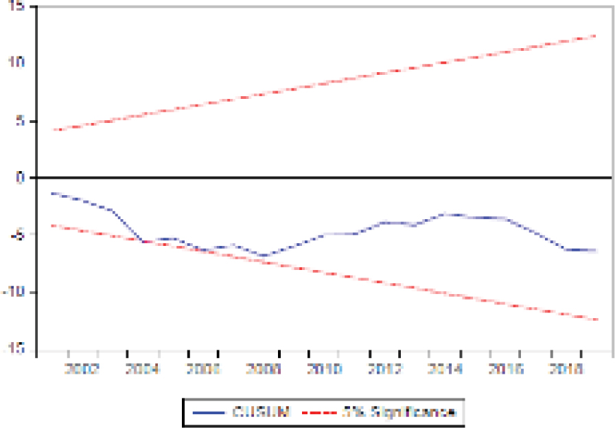
Figure 1:
Model stability: Cumulative sum of recursive residuals (CUSUM). Source: Output of EViews 10 software.
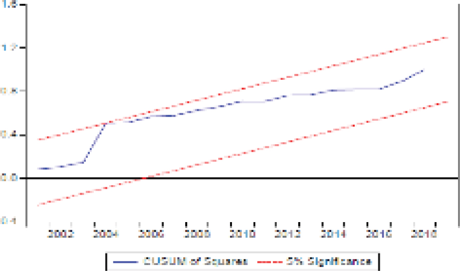
Figure 2:
Model stability: Cumulative sum of squares of recursive residuals (CUSUM of squares). Source: Output of EViews 10 software.