
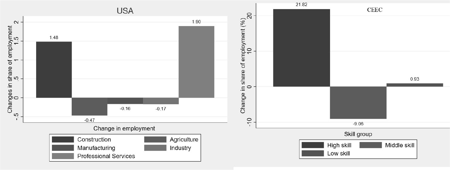
Figure 1
Job polarization in USA and CEEC, 2000–2016
Source: Generated by authors using data from the Bureau of Labour Statistics
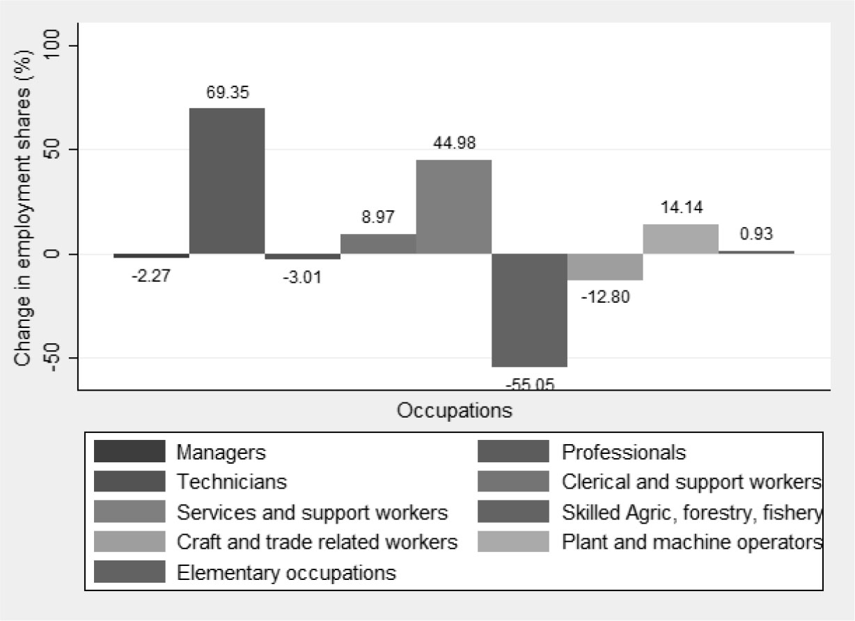
Figure 2
Employment performance by occupations in CEEC, 2000–2016
Source: Generated by authors using data from the Bureau of Labour Statistics
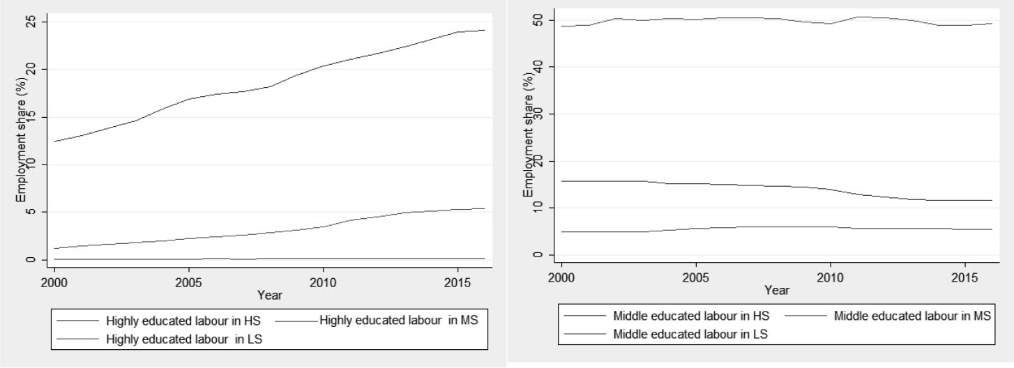
Figure 3
Labour in skill groups by education, CEEC
Source: Generated by authors using data from Eurostat
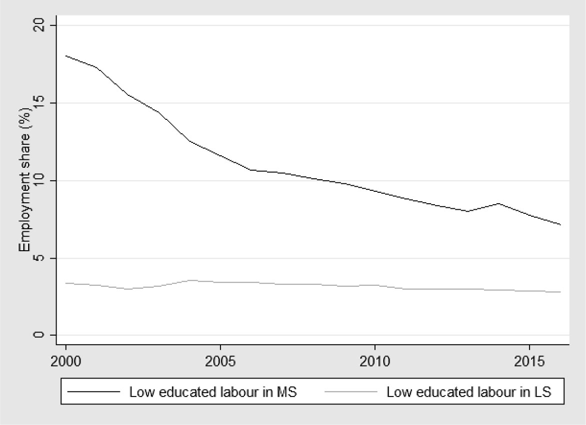
Figure 4
Lowly educated labour in other skill occupations, CEEC
Source: Generated by authors using data from Eurostat
Table 1
Results of Hausman test of mean group and pooled mean group models
| Low sill employment | ||||
| Variable | (b) | (B) | (b − B) | sqrt (diag (V_b − V_B)) |
| MG | PMG | difference | S.E. | |
| Log GVA(L1.) | 0.907 | 1.151 | −0.244 | 0.469 |
| Log TFP (L1.) | −2.422 | −3.569 | 1.147 | 3.926 |
| Chi2(2) = = (b − B)′ [(V _ b − V _ B) ˆ(−1)] (b − B) | P value | |||
| 0.4 | 0.821 | |||
| Middle skill employment | ||||
| Variable | (b) | (B) | (b − B) | sqrt diag (V _ b − V _ B) |
| MG | PMG | difference | S.E. | |
| Log GVA(L1.) | 0.228 | 0.428 | −0.200 | 0.090 |
| Log TFP (L1.) | −0.444 | −1.149 | 0.705 | 0.580 |
| Chi2(2) = = (b − B) ′ [(V _ b − V _ B) ˆ(−1)] (b − B) | P value | |||
| 4.94 | 0.085 | |||
| High skill employment | ||||
| Variable | (b) | (B) | (b − B) | sqrt diag (V _ b − V _ B) |
| MG | PMG | difference | S.E. | |
| Log GVA(L1.) | 0.009 | 0.205 | −0.197 | 0.273 |
| Log TFP (L1.) | 1.470 | 1.155 | 0.315 | 2.923 |
| Chi2(2) = = (b − B) ′ [(V _ b − V _ B) ˆ(−1)] (b − B) | P value | |||
| 4.94 | 0.085 | |||
[i] Note: b = consistent under Ho and Ha; obtained from xtpmg, B = inconsistent under Ha, efficient under Ho; obtained from xtpmg, Test: Ho: difference in coefficients not systematic, L1 represents lag 1, sqrt (square root)
[ii] Source: Generated by authors using STATA 15
Table 2
Impact of Technology on employment of low skill labour
| VARIABLES | ECT | Bulgaria | Czech R | Hungary | Poland | Romania | Slovakia |
|---|---|---|---|---|---|---|---|
| ECT | −0.559**(0.272) | 0.161**(0.090) | −0.109**(0.043) | −0.739***(0.135) | −0.543***(0.157) | −0.252**(0.109) | |
| D.Ln low skill | −0.68**(0.012) | −0.198***(0.002) | −0.56**(0.011) | −0.39***(0.009) | −0.18***(0.007) | −0.80**(0.091) | |
| D.ln GVA | −0.050(0.246) | −0.063(0.056) | −0.038(0.080) | 0.002(0.042) | 0.055(0.070) | 0.167(0.183) | |
| D.ln TFP | −0.999(2.002) | 1.007***(0.390) | 4.704**(1.915) | 2.433***(0.706) | 1.600***(0.523) | 1.168(0.852) | |
| D2.ln TFP | −0.975(2.171) | −0.521(0.539) | −4.181***(1.531) | −3.417***(0.918) | −2.555***(0.796) | −1.384(1.126) | |
| D3.ln TFP | 0.513(0.739) | 0.079(0.260) | 1.742***(0.676) | 0.831***(0.321) | 0.917***(0.352) | −0.115(0.531) | |
| L.ln GVA | 0.211***(0.068) | ||||||
| L.ln TFP | −2.882***(0.219) | ||||||
| Constant | 1.617*(0.869) | −0.428(0.306) | 0.267*(0.142) | 2.515***(0.802) | 1.890**(0.837) | 0.280(0.280) | |
| Observations | 72 | 72 | 72 | 72 | 72 | 72 | 72 |
[i] Note: The maximum number of lags for each variable was set to five. The optimal lag lengths were decided using the Akaike Information Criterion. The PMG estimators were computed by iterations obtained from xtpmg. Standard errors in parentheses, *** p < 0.01, ** p < 0.05, * p < 0.1, Standard errors in parentheses, *** p < 0.01, ** p < 0.05, * p < 0.1, Standard errors in parentheses, *** p < 0.01, ** p < 0.05, * p < 0.1, D, D2, D3 . . . Dn represent lags of first order difference variables. The variable L represents long-run, ECT (error correction term).
[ii] Source: Generated by authors using STATA 15
Table 3
Impact of Technology on middle skill labour
| VARIABLES | ECT | Bulgaria | Czech R | Hungary | Poland | Romania | Slovakia |
|---|---|---|---|---|---|---|---|
| ECT | −1.060***(0.210) | −0.209**(0.085) | −0.387**(0.021) | −0.372***(0.096) | −0.163***(0.051) | −0.195**(0.012) | |
| D.ln Middle Skill | −0.125**(0.055) | −0.190***(0.018) | −0.0170**(0.055) | −0.390***(0.004) | −0.220**(0.019) | −0.160**(0.032) | |
| D.ln GVA | 1.441***(0.243) | −0.292***(0.112) | 0.657*(0.350) | 0.492***(0.062) | 0.224***(0.057) | 0.470**(0.191) | |
| D2.ln GVA | −1.152***(0.286) | 0.446***(0.159) | −0.525(0.339) | −0.308***(0.072) | −0.053(0.069) | −0.051(0.230) | |
| D3.ln GVA | 0.473***(0.150) | −0.486***(0.105) | 0.193(0.134) | 0.034(0.040) | −0.066(0.041) | −0.071(0.105) | |
| D.ln TFP | −0.006(0.011) | −0.161***(0.034) | 0.014(0.050) | −0.015(0.018) | −0.038***(0.013) | 0.006(0.021) | |
| L. ln GVA | 0.368***(0.065) | ||||||
| L.ln TFP | −0.719***(0.187) | ||||||
| Constant | 3.588***(0.736) | 0.613*(0.325) | 1.246(0.839) | 1.589***(0.464) | 0.607**(0.261) | 0.589(0.432) | |
| Observations | 72 | 72 | 72 | 72 | 72 | 72 | 72 |
| Standard errors in parentheses *** p < 0.01, ** p < 0.05, * p < 0.1 | |||||||
[i] Note: The maximum number of lags for each variable was set to five. The optimal lag lengths were decided using the Akaike Information Criterion. The PMG estimators were computed by iterations obtained from xtpmg. Standard errors in parentheses, *** p < 0.01, ** p < 0.05, * p < 0.1, Standard errors in parentheses, *** p < 0.01, ** p < 0.05, * p < 0.1, Standard errors in parentheses, *** p < 0.01, ** p < 0.05, * p < 0.1, D, D2, D3 . . . Dn represent lags of first order difference variables. The variable L represents long-run, ECT (error correction term).
[ii] Source: Generated by authors using STATA 15
Table 4
Impact of Technology on high skill labour
| VARIABLES | ECT | Bulgaria | Czech R | Hungary | Poland | Romania | Slovakia |
|---|---|---|---|---|---|---|---|
| ECT | 0.100**(0.0145) | −0.923***(0.138) | −0.55***(0.034) | −0.850***(0.180) | −0.383***(0.060) | −0.969***(0.268) | |
| D.ln High skill | −0.124**(0.048) | −0.48**(0.020) | −0.21**(0.020) | −0.47(0.029) | −0.50***(0.003) | −0.70**(0.036) | |
| D.ln GVA | −0.551(0.429) | 1.053***(0.169) | −0.301***(0.104) | 0.194(0.180) | 0.279***(0.029) | −1.834***(0.550) | |
| D2.ln GVA | 1.585***(0.597) | −2.725***(0.487) | 0.948***(0.302) | −0.257(0.273) | −0.196***(0.068) | 4.396***(1.443) | |
| D3.ln GVA | −2.030**(0.798) | 3.312***(0.693) | −0.768**(0.385) | 0.416(0.283) | 0.617***(0.094) | −3.966***(1.366) | |
| D4.ln GVA | 1.143*(0.592) | −1.655***(0.420) | 0.163(0.222) | −0.215(0.150) | −0.804***(0.070) | 1.916***(0.691) | |
| D5.ln GVA | −0.237(0.189) | 0.311***(0.098) | 0.001(0.052) | 0.041(0.034) | 0.298***(0.021) | −0.389***(0.142) | |
| D.TFP | −0.176(0.300) | 1.634***(0.356) | 0.010(0.185) | 1.100***(0.319) | −0.440***(0.090) | 0.964**(0.442) | |
| L.ln GVA | 0.213***(0.025) | ||||||
| L.TFP | 2.560***(0.181) | ||||||
| Constant | −0.197(0.358) | 3.320***(0.484) | 0.201*(0.103) | 3.220***(0.679) | 1.290***(0.224) | 2.214***(0.606) | |
| Observations | 72 | 72 | 72 | 72 | 72 | 72 | 72 |
| Standard errors in parentheses *** p < 0.01, ** p < 0.05, * p < 0.1 | |||||||
[i] Note: The maximum number of lags for each variable was set to five. The optimal lag lengths were decided using the Akaike Information Criterion. The PMG estimators were computed by iterations obtained from xtpmg. Standard errors in parentheses, *** p < 0.01, ** p < 0.05, * p < 0.1, Standard errors in parentheses, *** p < 0.01, ** p < 0.05, * p < 0.1, Standard errors in parentheses, *** p < 0.01, ** p < 0.05, * p < 0.1, D, D2, D3 . . . Dn represent lags of first order difference variables. The variable L represents long-run, ECT (error correction term).
[ii] Source: Generated by authors using STATA 15