

Figure 1.
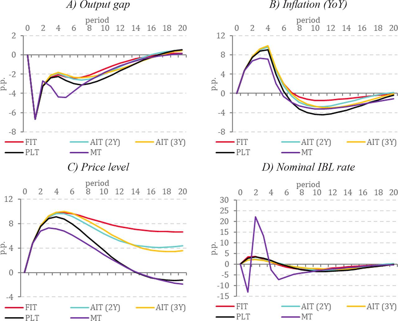
Figure 2.
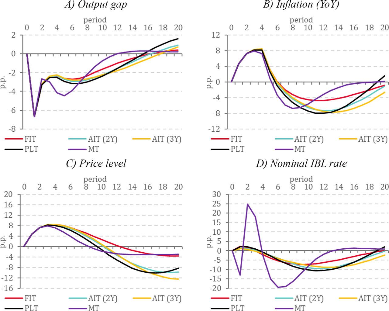
Figure 3.
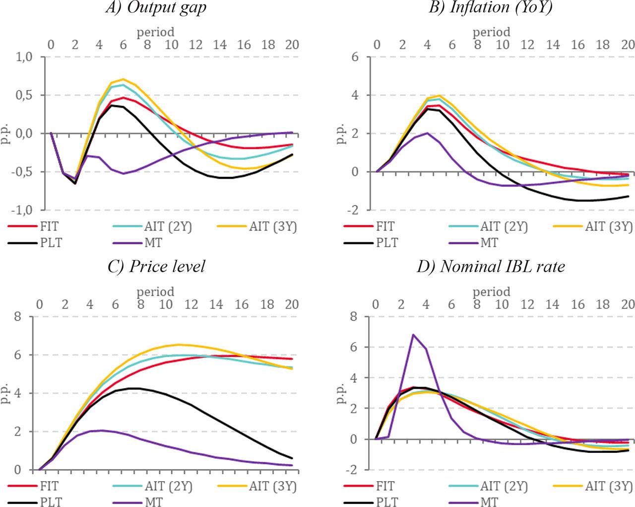
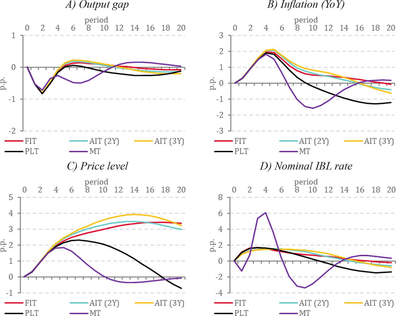
Figure 4.
Values of key model parameters
| Parameter | Value | Parameter | Value |
|---|---|---|---|
| Output gap | Core inflation | ||
| a1 | 0.55 | b1 | 0.35 |
| a2 | 0.05 | b2 | 0.09 |
| a3 | 0.20 | b3 | 0.20 |
| a4 | 0.35 | Real marginal costs | |
| a5 | 0.10 | k1 | 0.45 |
| a6 | 0.15 | k2 | 0.25 |
| Wages | Non-core inflation | ||
| aa1 | 0.55 | bb1 | 0.60 |
| aa2 | 0.40 | bb2 | 0.05 |
| aa3 | 0.25 | bb3 | 0.10 |
| Exports | Imports | ||
| c1 | 0.45 | d1 | 0.40 |
| c2 | 0.45 | d2 | 1.00 |
| c3 | 0.25 | d3 | 0.10 |
| Exchange rate | Monetary policy reaction function | ||
| h1 | 0.30 | mm1 | 0.60 |
| h2 | 0.90 | mm2 | 0.55 |
| Monetary conditions | mm3 | 0.30 | |
| m1 | 0.50 | ||
| m2 | 0.15 | ||
| m3 | 0.35 | ||
Simulation results of a scenario of worsening external economic conditions: Baseline model specification
| Indicator | Monetary policy regime | ||||
|---|---|---|---|---|---|
| FIT | AIT (2Y) | AIT (3Y) | PLT | MT | |
| σ(ŷ) | 0.4 | 0.4 | 0.5 | 0.4 | 0.4 |
| σ(π4) | 2.1 | 2.3 | 2.5 | 1.9 | 1.1 |
| σ(p) | 4.4 | 4.8 | 5.1 | 3.5 | 1.5 |
| σ(∆i) | 0.7 | 0.6 | 0.6 | 0.7 | 1.7 |
| L(γ=0.25) | 12.3 | 14.2 | 16.2 | 8.0 | 2.6 |
| L(γ=0.50) | 12.5 | 14.3 | 16.3 | 8.1 | 3.3 |
| L(γ=0.75) | 12.6 | 14.4 | 16.4 | 8.3 | 4.1 |
Simulation results of a scenario of worsening domestic economic conditions: Baseline model specification
| Indicator | Monetary policy regime | ||||
|---|---|---|---|---|---|
| FIT | AIT (2Y) | AIT (3Y) | PLT | MT | |
| σ(ŷ) | 2.8 | 2.9 | 2.8 | 3.2 | 3.5 |
| σ(π4) | 5.0 | 5.1 | 5.2 | 5.3 | 4.4 |
| σ(p) | 8.5 | 7.7 | 8.1 | 6.5 | 5.3 |
| σ(∆i) | 1.2 | 0.8 | 0.7 | 1.1 | 12.1 |
| L(γ=0.25) | 52.8 | 47.5 | 50.8 | 40.7 | 66.3 |
| L(γ=0.50) | 53.2 | 47.7 | 50.9 | 41.0 | 103.0 |
| L(γ=0.75) | 53.6 | 47.8 | 51.1 | 41.3 | 139.7 |
Simulation results of a scenario of worsening external economic conditions: Strict restrictions on capital flows
| Indicator | Monetary policy regime | ||||
|---|---|---|---|---|---|
| FIT | AIT (2Y) | AIT (3Y) | PLT | MT | |
| σ(ŷ) | 0.3 | 0.3 | 0.3 | 0.3 | 0.4 |
| σ(π4) | 1.2 | 1.3 | 1.3 | 1.1 | 1.2 |
| σ(p) | 2.4 | 2.6 | 2.8 | 1.9 | 1.1 |
| σ(∆i) | 0.4 | 0.3 | 0.3 | 0.4 | 2.1 |
| L(γ=0.25) | 3.7 | 4.3 | 4.8 | 2.4 | 2.6 |
| L(γ=0.50) | 3.7 | 4.3 | 4.9 | 2.5 | 3.7 |
| L(γ=0.75) | 3.8 | 4.3 | 4.9 | 2.5 | 4.8 |
Simulation results of a scenario of worsening domestic economic conditions: Strict restrictions on capital flows
| Indicator | Monetary policy regime | ||||
|---|---|---|---|---|---|
| FIT | AIT (2Y) | AIT (3Y) | PLT | MT | |
| σ(ŷ) | 2.9 | 3.1 | 3.1 | 3.2 | 3.3 |
| σ(π4) | 5.2 | 6.0 | 5.9 | 6.3 | 5.7 |
| σ(p) | 6.0 | 5.7 | 5.8 | 5.6 | 4.7 |
| σ(∆i) | 1.3 | 1.1 | 1.0 | 1.4 | 13.9 |
| L(γ=0.25) | 35.9 | 39.3 | 39.5 | 41.3 | 80.6 |
| L(γ=0.50) | 36.3 | 39.6 | 39.7 | 41.8 | 128.8 |
| L(γ=0.75) | 36.8 | 40.0 | 40.0 | 42.3 | 177.0 |
Efficiency of monetary policy regimes in an unconditional simulation experiment: Baseline model specification
| Indicator | Monetary policy regime | ||||
|---|---|---|---|---|---|
| FIT | AIT (2Y) | AIT (3Y) | PLT | MT | |
| (γ=0.25) | 2.3 | 3.6 | 4.7 | 1.6 | 2.8 |
| L(γ=0.50) | 2.1 | 3.4 | 4.5 | 1.5 | 3.5 |
| L(γ=0.75) | 2.1 | 3.4 | 4.2 | 1.5 | 3.8 |
Efficiency of monetary policy regimes in an unconditional simulation experiment: Strict restrictions on capital flows
| Indicator | Monetary policy regime | ||||
|---|---|---|---|---|---|
| FIT | AIT (2Y) | AIT (3Y) | PLT | MT | |
| (γ=0.25) | 2.7 | 3.9 | 4.9 | 1.7 | 1.8 |
| L(γ=0.50) | 2.4 | 3.7 | 4.7 | 1.6 | 2.6 |
| L(γ=0.75) | 2.3 | 3.6 | 4.5 | 1.5 | 3.1 |